- Related AI/ML Methods: Multivariate Discriminant Analysis (LDA), Random Forest
- Related Traditional Methods: Linear Discriminant Analysis
The Classification and Regression Trees (CART) model generates branches and subgroups of the categorical dependent Y variable using characteristic X variables. CART is typically used for data mining and constitutes a supervised machine learning approach. This is a classification approach when the dependent variable is categorical, and the tree is used to determine the class or group within which a target testing variable is most likely to fall. The data is split into branches along a tree, and each branch split will be determined using Gini coefficients and information loss coefficients based on the questions asked along the way. Specifically, ![]() . If this Gini index is 0, it means the data are perfectly classified. Therefore, using a recursive algorithm, we can apply the splits that have the lowest Gini index. The final structure looks like a tree with its many branches. Additional splitting and stopping rules are applied along the way, and the terminal branches will provide predictions of the target testing variable.
. If this Gini index is 0, it means the data are perfectly classified. Therefore, using a recursive algorithm, we can apply the splits that have the lowest Gini index. The final structure looks like a tree with its many branches. Additional splitting and stopping rules are applied along the way, and the terminal branches will provide predictions of the target testing variable.
Figure 9.57 provides a visual illustration and the results of a CART model. Simply enter the variables you need to classify and enter the number of clusters desired. The CART model then generates if-then-else rules that are simple to understand and implement as a forecasting tool. The tree can identify patterns that are oftentimes obscured in the complex interactions of the data.
The CART algorithm runs the optimal splits according to the Gini coefficient and then retests the regression tree against the actual Training ![]() variable to identify its accuracy. If a different set of Testing
variable to identify its accuracy. If a different set of Testing ![]() variables is entered, it will also project and classify the relevant groupings (Figure 9.58). The sample data shows the information on 10 individuals, where each individual’s preferred transportation mode is the dependent variable (a categorical variable 1, 2, 3 for bus, train, or car). The independent predictors are the individuals’ gender (1, 2 for male or female), whether the person owns a car (1, 0 for yes or no), the cost of transportation (1, 2, 3 for cheap, medium, or expensive), and the individual’s income level category (1, 2, 3 for low, medium, or high). Back in Figure 9.57, we see the tree visually, with all the relevant splits and Gini coefficients. The tree is then used to back-fit the original data. For the example data (Figure 9.58), the first individual who ended up taking the Bus (Transportation Mode = 1) has the following dependent variable values: Gender = 1, Car Ownership = 0, Transportation Cost = 1, and Income Level = 1. We start from the top of the tree in Figure 9.57 and see that for cost = 1, we take the first right branch, then going down the next level, we take the right branch where travel cost = 1. Then, we take the left branch where gender = 1. The path is bolded for easier identification. This happens to be the terminal branch, which means the model predicts that the transport mode is 1, corresponding to the original data. All rows of data are fed through this tree according to their own pathways.
variables is entered, it will also project and classify the relevant groupings (Figure 9.58). The sample data shows the information on 10 individuals, where each individual’s preferred transportation mode is the dependent variable (a categorical variable 1, 2, 3 for bus, train, or car). The independent predictors are the individuals’ gender (1, 2 for male or female), whether the person owns a car (1, 0 for yes or no), the cost of transportation (1, 2, 3 for cheap, medium, or expensive), and the individual’s income level category (1, 2, 3 for low, medium, or high). Back in Figure 9.57, we see the tree visually, with all the relevant splits and Gini coefficients. The tree is then used to back-fit the original data. For the example data (Figure 9.58), the first individual who ended up taking the Bus (Transportation Mode = 1) has the following dependent variable values: Gender = 1, Car Ownership = 0, Transportation Cost = 1, and Income Level = 1. We start from the top of the tree in Figure 9.57 and see that for cost = 1, we take the first right branch, then going down the next level, we take the right branch where travel cost = 1. Then, we take the left branch where gender = 1. The path is bolded for easier identification. This happens to be the terminal branch, which means the model predicts that the transport mode is 1, corresponding to the original data. All rows of data are fed through this tree according to their own pathways.
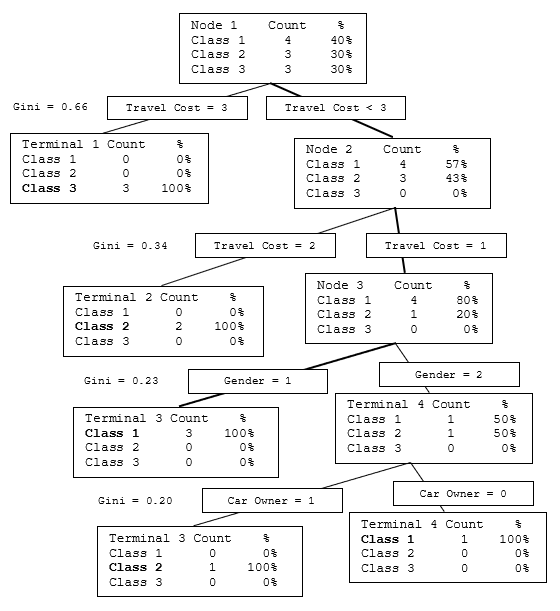
Figure 9.57: Classification and Regression Tree (CART)
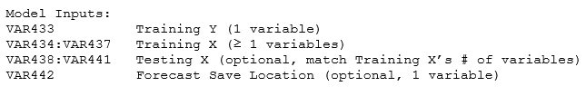
The required model inputs look like the following:
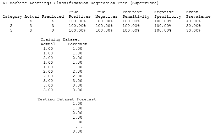
The complete results from the algorithm are shown next. The CART method will return the various unique numerical categories in the Training ![]() set, and, in this example, we have three categories: 1, 2, and 3. It will show the fit of the training dataset, where here we see the actuals versus CART predicted results, with a perfect 100% accuracy match in each category. The actual categories based on the training set are shown, together with the model’s predicted categorization. This fitted model and its comparison to actuals allow one to see the accuracy of the model. Then, using this fitted model, if the optional Testing
set, and, in this example, we have three categories: 1, 2, and 3. It will show the fit of the training dataset, where here we see the actuals versus CART predicted results, with a perfect 100% accuracy match in each category. The actual categories based on the training set are shown, together with the model’s predicted categorization. This fitted model and its comparison to actuals allow one to see the accuracy of the model. Then, using this fitted model, if the optional Testing ![]() variables are provided, the algorithm takes this testing dataset and computes the predicted categories.
variables are provided, the algorithm takes this testing dataset and computes the predicted categories.
The interpretation of True Positive (TP), False Negatives (FN), False Positives (FP), and True Negatives (TN) are best shown in the table below. Positive Sensitivity Recall measures the ability to predict positive outcomes while Negative Specificity measures the ability to predict negative outcomes. Event Prevalence is the percentage of each category in the training dataset. Finally, Overall Accuracy is the overall prediction is both TP and TN as a proportion of the original training dataset.
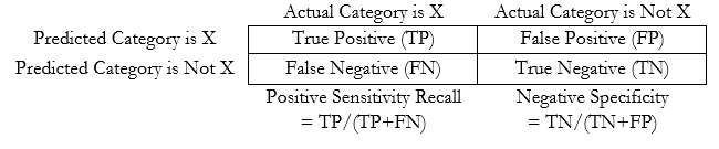
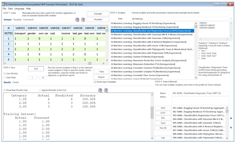
Figure 9.58: AI/ML Classification and Regression Tree CART