Payback Period (PP)
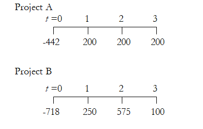
Suppose you are to choose between two projects, A and B. Project A costs $442 but pays back $200 for the next 3 years, while B costs $718 and pays back $250, $575, and $100 for the next 3 years.
The manual calculations are shown below and in Figure 1.1.
Payback A is between years 2 and 3,as -$442 pays back between $200+$200 in year 2 and $200+$200+$200 in year 3
2 years is $200+$200 or $400 paid back, with $442-$400 =$42 remaining to be paid back in year 3
Payback A = 2 + [$42÷$200] = 2.21 years
Payback B is between years 1 and 2,as -$718 pays back between $250 in year 1 and $250+$575 in year 2
1 year is $250 paid back, with $718-$250 remaining to be paid back in year 2
Payback B = 1 + [($718-$250)÷ $575] = 1.81 years
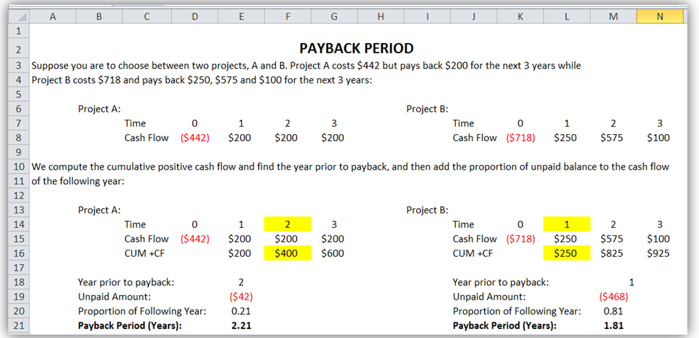
Figure 1.1: Payback Period Manual Computations
Disadvantages of Payback Period
- Neglects time value of money. To solve this, use present values instead of cash flows, that is, use a discounted payback period instead. This means that in the example above, the $200, or $250, $575, and $100 cash flows are first discounted to present values. See the Discounted Payback Period example below.
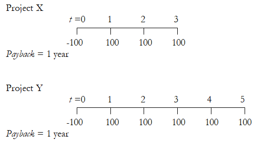
- Cash flows and length of time remaining are left out after the payback period. As an example, suppose we have two new projects, X and Y with cash flows as shown below. Both have identical payback periods but clearly, project Y is superior as it has additional cash flows. These cash flows post payback period are ignored.
Discounted Payback Period (DPP)
Suppose you are to choose between two projects, A and B. Project A costs $442 but pays back $200 for the next 3 years, while B costs $718 and pays back $250, $575, and $100 for the next 3 years. Further suppose that the WACC discount rate is 12%. The manual computations are shown below and in Figure 1.2.
Discounted Payback A = 2 + [($442-$338.0)÷ $142.4] = 2.73 years
Discounted Payback B = 2 + [($718-$681.6)÷ $71.2] = 2.51 years
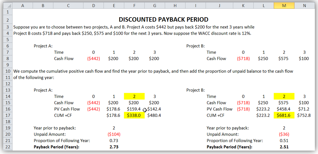
Figure 1.2: Discounted Payback Period Manual Computations
Net Present Value (NPV)
Using the projects A and B below, which project is better assuming a 12% WACC discount rate? Use the NPV method.
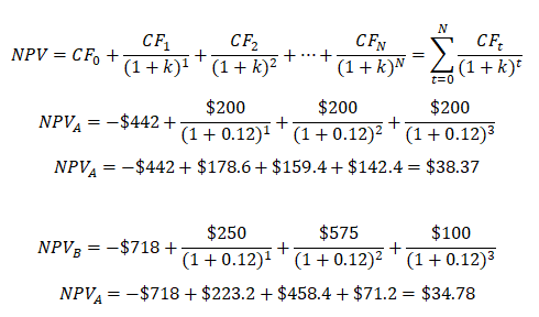
Comparing A and B, A has a higher NPV, therefore A should be chosen before B although both projects should be undertaken if there exist sufficient funds, otherwise, only undertake project A. Rank remains the same but NPV values differ using different discount rates. Figure 1.3 shows the computations in Excel using the NPV function. Please note that Excel’s NPV function starts from Year 1, which means you need to set the function for cash flows from Years 1 to N, and add the cash flow of Year 0, as illustrated in Figure 1.3’s two NPV functions.
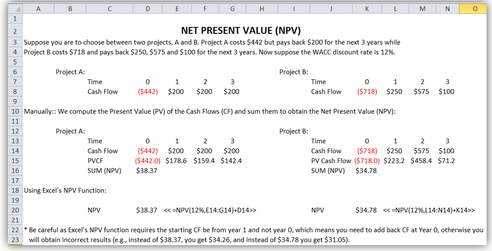
Figure 1.3: Net Present Value Manual Computations
Internal Rate of Return (IRR)
Using the same scenario above, calculate the IRR for projects A and B assuming a 12% WACC discount rate (this will now be used as the hurdle rate). Should we accept both projects again, and which project is better?
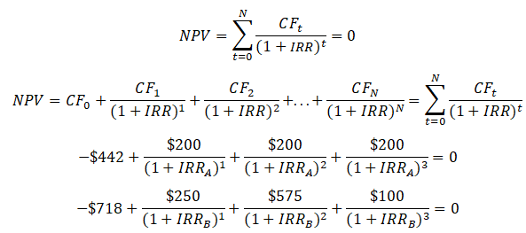
Using trial and error, simple optimization, or search function (Goal Seek in Excel), we obtain IRR for project A to be 16.99% and 14.99% for project B. The decision should be to choose Project A over B as it has a higher return (IRR) and IRR > k for both. Figure 1.4 shows the annual computations of IRR using Excel’s IRR function (unlike the NPV function that starts with Year 1 cash flow, the IRR function starts with Year 0’s cash flow as illustrated in the figure).
Multiple Internal Rate of Returns
When cash flows are both + and –, there may exist multiple IRRs. For instance, consider a project costing –$1.6M with returns of +$10M in the first year and a loss of –$10M in the second year. What is the project’s IRR?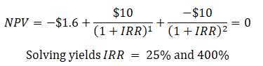
The conclusion is that one should use all methods at one’s disposal and see which makes more sense. In regular situations, they should all have similar results. Figure 1.5 shows how multiple IRR errors can exist with a simple fluctuating cash flow.
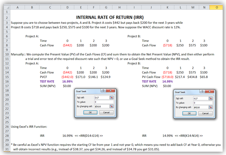
Figure 1.4: Internal Rate of Return Manual Computations
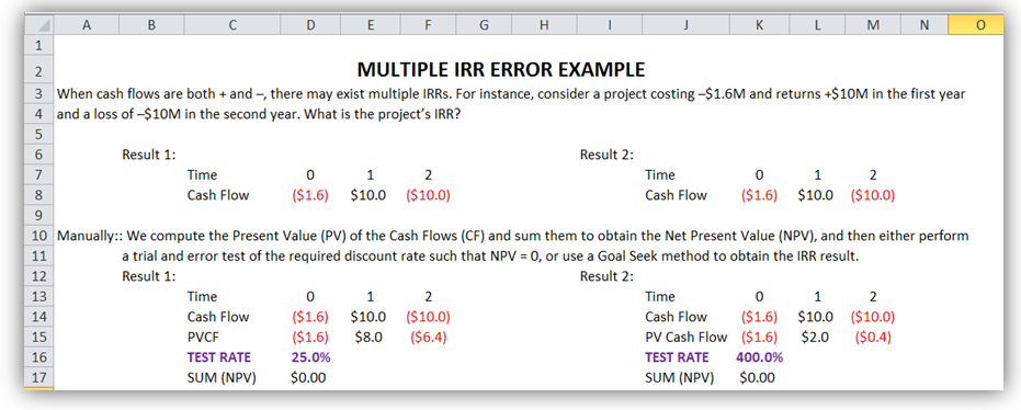
Figure 1.5: Multiple IRR Error
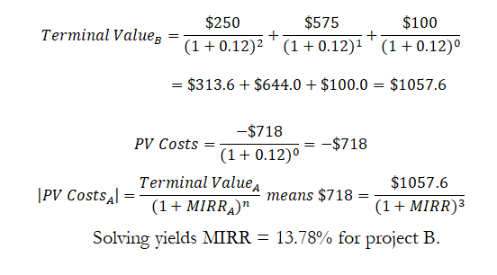
Modified Internal Rate of Return (MIRR)
Calculate the MIRR for the two projects A and B as specified previously. Figure 1.6 shows the manual computations of the modified internal rate of return (MIRR) using cash out-flows (COF) and cash in-flows (CIF):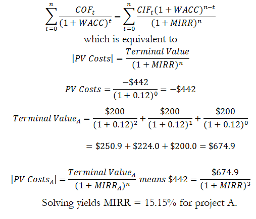
Profitability Index and Return on Investment (PI and ROI)
Compute the profitability index (PI) and return on investment (ROI) on Projects A and B as previously specified. Figure 1.7 shows the manual computation of the PI and ROI.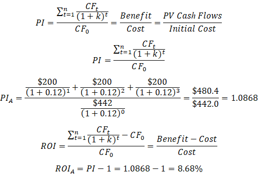
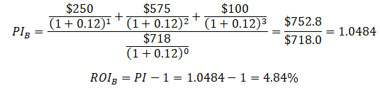
We see that ROI and PI of project A exceeds that of project B, so we would recommend going ahead with project A instead of project B.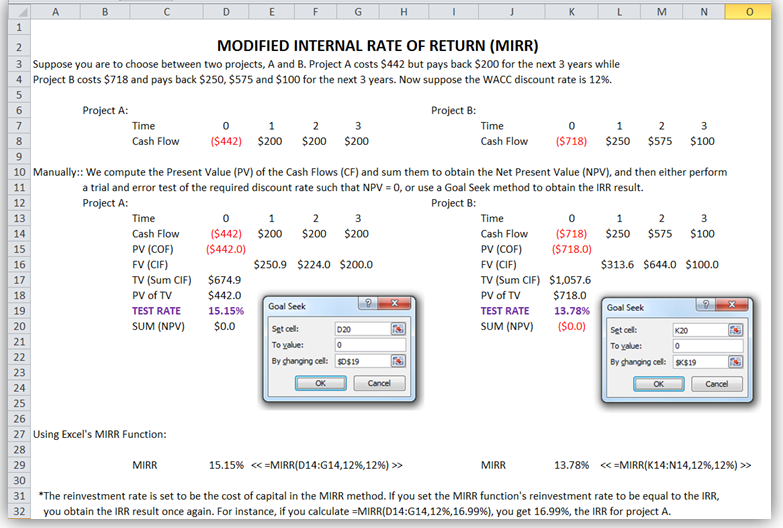
Figure 1.6: Modified Internal Rate of Return Manual Computations
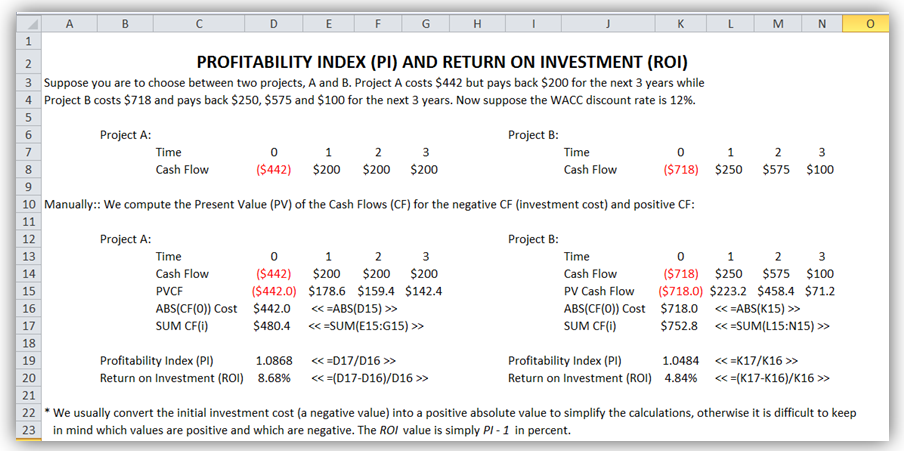
Figure 1.7: Profitability Index and Return on Investment Manual Computations