File Name: Forecasting – Logistic S-Growth Curves
Location: Modeling Toolkit | Forecasting | Logistic S-Growth Curves
Brief Description: Illustrates how to run a simulation model on the logistic S-growth curve where the growth rate is uncertain over time, to determine the probabilistic outcomes at some point in the future
Requirements: Modeling Toolkit, Risk Simulator
A logistic function or logistic curve models the S curve of growth of some variable. The initial stage of growth is approximately exponential; then, as competition arises, growth slows, and at maturity, growth stops (Figure 85.1). These functions find applications in a range of fields, from biology to economics. For example, in the development of an embryo, a fertilized ovum splits, and the cell count grows 1, 2, 4, 8, 16, 32, 64, etc. This is exponential growth. But the fetus can grow only as large as the uterus can hold; thus other factors start slowing down the increase in the cell count, and the rate of growth slows (but the baby is still growing, of course). After a suitable time, the child is born and keeps growing. Ultimately, the cell count is stable; the person’s height is constant; the growth has stopped at maturity. The same principles can be applied to the population growth of animals or humans, and the market penetration and revenues of a product, where there is an initial growth spurt in market penetration, but over time, the growth slows due to competition, and eventually the market declines and matures.
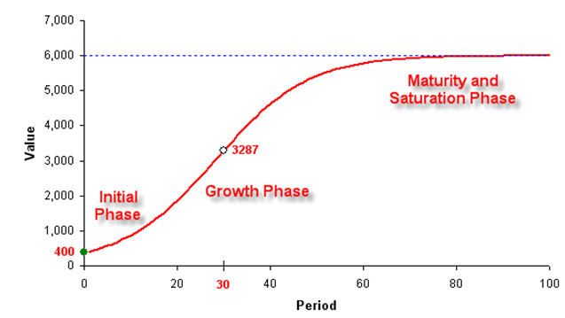
Figure 85.1: Logistic S curve
Procedure
You can run the preset simulation by clicking on Risk Simulator | Change Profile and selecting the S Curve profile, then run the simulation by going to Risk Simulator | Run Simulation. Alternatively, you can set your own or change the underlying simulation assumption as well as the input parameters. The Growth Rate, Maximum Capacity, and Initial Value are the input values in the model to determine the characteristics of the S curve. In addition, you can also enter in the Lookup Year to determine the value for that particular year, where the corresponding value for that year is set as a forecast. Using the initial model inputs and running the simulation yields the forecast charts seen in Figure 85.2, where the expected value of Year 30 is 2054.88 units.
Alternatively, you can use Risk Simulator’s S-curve forecasting module to automatically generate forecast values (Risk Simulator | Forecasting | JS Curves).
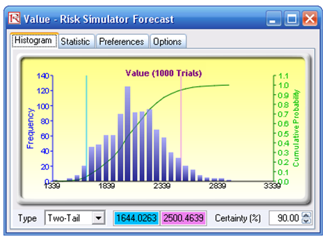
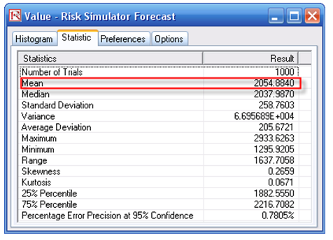
Figure 85.2: Simulated results on the logistic S curve