File Name: Analytics – Flaw of Averages
Location: Modeling Toolkit | Analytics | Flaw of Averages
Brief Description: Illustrates the concept of the Flaw of Averages (where using the simple average sometimes yields incorrect answers) through the introductions of harmonic averages, geometric averages, medians, and skew
Requirements: Modeling Toolkit
This model does not require any simulations or sophisticated modeling. It is simply an illustration of various ways to look at the first moment of a distribution (measuring the central tendency and location of a distribution), that is, the mean or average value of a distribution or data points. This model shows how a simple arithmetic average can be wrong in certain cases and how harmonic averages, geometric averages, and medians are sometimes more appropriate.
Flaw of Averages: Geometric Average
Suppose you purchased a stock at some time period (call this time zero) for $100. Then, after one period (e.g., a day, a month, a year), the stock price goes up to $200 (period one), at which point you should sell and cash in the profits, but you do not, and hold it for another period. Further suppose that at the end of period two, the stock price drops back down to $100, and then you decide to sell. Assuming there are no transaction costs or hidden fees for the sake of simplicity, what is your average return for these two periods?
Period Stock Price
0 $100
1 $200
2 $100
First, let’s compute it the incorrect way, using arithmetic averages:
Absolute Return from Period 0 to Period 1: 100%
Absolute Return from Period 1 to Period 2: -50%
Average Return for both periods: 25%
That is, the return for the first holding period is (New – Old)/Old or ($200 – $100)/$100 = 100%, which makes sense as you started with $100, and it then became $200 or returned 100%. Next, the second holding period return is ($100 – $200)/$200 = –50%, which also makes sense as you started with $200 and ended up with $100 or lost half the value. So, the arithmetic average of 100% and –50% is (100% + [–50%])/2 = 25%.
Well, clearly you did not make 25% in returns. You started with $100 and ended up with $100. How can you have a 25% average return? So, this simple arithmetic mean approach is incorrect. The correct methodology is to use geometric average returns, applying something called relative returns:
Period Stock Price Relative Returns
0 $100
1 $200 2.00
2 $100 0.50
Absolute returns are similar to relative returns, less one. For instance, going from $10 to $11 implies an absolute return of ($11–$10)/$10 = 10%. However, using relative returns, we have $11/$10 = 1.10. If you take 1 off this value, you obtain the absolute returns. Also, 1.1 means a 10% return and 0.9 means a –10% return, and so forth. The preceding table shows the computations of the two relative returns for the two periods. We then compute the geometric average where we have: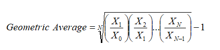
That is, we take the root of the total number of periods N of the multiplications of the relative returns. We then obtain a geometric average of 0.00%.
Alternatively, we can use Excel’s equation of “=POWER(2.00*0.50,1/2)–1” to obtain 0%. Note that the POWER function in Excel takes X to some power Y in “POWER (X,Y)”; the root of 2 (N is 2 periods in this case, not including period 0) is the same as taking it to the power of 1/2.
This 0% return on average for the periods make a lot more sense. Be careful when you see large stock or fund returns as some may actually be computed using arithmetic averages. Where there is an element of time series in the data and fluctuations of the data are high in value, be careful when computing the series’ average as the geometric average might be more appropriate.
Note: For simplicity, you can also use Excel’s GEOMEAN function on the relative returns and deduct one from it. Note that you have to take the GEOMEAN of the relative returns: =GEOMEAN(2,0.5)-1 and minus one, not the raw stock prices themselves.
Flaw of Averages: Harmonic Average
Say there are three people, Larry, Curly, and Moe, who happen to be cycling enthusiasts, apart from being movie stars and close friends. Further, suppose each one has a different level of physical fitness, and they ride their bikes at a constant speed of 10 miles per hour (mph), 20 mph, and 30 mph, respectively.
Biker Constant Miles/Hour
Larry 10
Curly 20
Moe 30
The question is, how long will it take on average for all three cyclists to complete a 10-mile course? Well, let’s first solve this problem the incorrect way, in order to understand why it is so easy to commit the Flaw of Averages. First, computing it the wrong way, we obtain the average speed of all three bikers, that is, (10 + 20 + 30)/3 = 20 mph. So, according to that calculation, it would take 10 miles/20 miles per hour = 0.5 hours to complete the trek on average.
Biker Constant Miles/Hour
Larry 10
Curly 20
Moe 30
Average 20 miles/hour
Distance 10 miles
Time to complete the 0.5 hours
10-mile trek
By doing this, we are committing a serious mistake. The average time is not the 0.5 hours figured by using the simple arithmetic average. Let us prove why this is the case. First, let’s show the time it takes for each biker to complete 10 miles. Then we simply take the average of these times.
Biker Constant Miles/Hour Time to Complete 10 miles
Larry 10 1.00 hours
Curly 20 0.50 hours
Moe 30 0.33 hours
Average 0.6111 hours
So, the true average is actually 0.6111 hours or 36.67 minutes, not 30 minutes or 0.5 hours. How do we compute the true average?
The answer lies in the computation of harmonic averages, where we define the harmonic average as 
where N is the total number of elements, in this case, 3; and Xi are values of the individual elements. That is, we have the following computations:
Biker Constant Miles/Hour
Larry 10
Curly 20
Moe 30
N 3.0000
SUM (1/X) 0.1833
Harmonic 16.3636
Arithmetic 20.0000
Therefore, the harmonic average speed of 16.3636 mph would mean that a 10-mile trek would take 10/16.3636 or 0.6111 hours (36.67 minutes). Using a simple arithmetic average would yield wrong results when you have rates and ratios that depend on time.
Flaw of Averages: Skewed Average
Assume that you are in a room with 10 colleagues, and you are tasked with figuring out the average salary of the group. You start to ask around the room to obtain 10 salary data points, and then quantify the group’s average:
Person Salary
1 $75,000
2 $120,000
3 $95,000
4 $69,800
5 $72,000
6 $75,000
7 $108,000
8 $115,000
9 $135,000
10 $100,000
Average $96,480
This average is, of course, the arithmetic average or the sum of all the individual salaries divided by the number of people present.
Suddenly, a senior executive enters the room and participates in the little exercise. His salary, with all the executive bonuses and perks, came to $20 million last year. What happens to your new computed average?
Person Salary
1 $75,000
2 $120,000
3 $95,000
4 $69,800
5 $72,000
6 $75,000
7 $108,000
8 $115,000
9 $135,000
10 $100,000
11 $20,000,000
Average $1,905,891
The average now becomes $1.9 million. This value is clearly not representative of the central tendency and the “true average” of the distribution. Looking at the raw data, to say that the average salary of the group is $96,480 per person makes more sense than $1.9 million per person.
What happened? The issue was that an outlier existed. The $20 million is an outlier in the distribution, skewing the distribution to the right. When there is such an obvious skew, the median would be a better measure as the median is less susceptible to outliers than the simple arithmetic average.
Median for 10 people: $97,500
Median for 11 people: $100,000
Thus, $100,000 is a much better representative of the group’s “true average.”
Other approaches exist to find the “true” or “truncated” mean. They include performing a single variable statistical hypothesis t-test on the sample raw data or simply removing the outliers. However, be careful when dealing with outliers; sometimes outliers are very important data points. For instance, extreme stock price movements actually may yield significant information. These extreme price movements may not be outliers but, in fact, are part of doing business, as extreme situations exist (i.e., the distribution is leptokurtic, with a high kurtosis) and should be modeled if the true risk profile is to be constructed.
Another approach to spot an outlier is to compare the mean with the median. If they are very close, the distribution is probably symmetrically distributed. If the mean and median are far apart, the distribution is skewed, and a skewed mean is typically a bad approximation of the true mean of the distribution. Care should be taken when you spot a high positive or negative skew. You can use Excel’s SKEW function to compute the skew:
Skew for 10 people: 0.28
Skew for 11 people: 3.32
As expected, the skew is high for the 11-person group as there is an outlier and the difference between the mean and median is significant.