File Names: Six Sigma – Sample Size Correlation; Six Sigma – Sample Size DPU; Six Sigma – Sample Size Mean; Six Sigma – Sample Size Proportion; Six Sigma – Sample Size Sigma, Six Sigma – Delta Precision; Six Sigma – Design of Experiments and Combinatorics
Location: Modeling Toolkit | Six Sigma
Brief Description: Illustrate how to obtain the required sample size in performing hypotheses testing from means to standard deviations and proportions
Requirements: Modeling Toolkit, Risk Simulator
Modeling Toolkit Functions Used: MTSixSigmaSampleSize, MTSixSigmaSampleSizeProportion, MTSixSigmaSampleSizeZeroCorrelTest, MTSixSigmaSampleSizeDPU, MTSixSigmaSampleSizeStdev, MTSixSigmaDeltaPrecision
In performing quality controls and hypothesis testing, the size of the samples collected is of paramount importance. Theoretically, it would be impossible or too expensive and impractical to collect information and data on the entire population to be tested (e.g., all outputs from a large manufacturing facility). Therefore, statistical sampling is required. The question is: What size sample is sufficient? The size of a statistical sample is the number of repeated measurements that are collected. It is typically denoted n, a positive integer. Sample size determination is critical in Six Sigma and quality analysis as different sample sizes lead to different accuracies and precision of measurement. This can be seen in such statistical rules as the Law of Large Numbers and the Central Limit Theorem. With all else being equal, a larger sample size n leads to increased precision in estimates of various properties of the population. The question that always arises is: How many sample data points are required? The answer is: it depends. It depends on the error tolerances and precision required in the analysis. This model is used to compute the minimum required sample size given the required error, precision, and variance levels.
There are five different sample size determination models in the Modeling Toolkit. The first model (Six Sigma – Sample Size Mean) computes the minimum required sample size for a hypothesis test (one- or two-tailed test), where the required errors and precisions are stated, as is the sample standard deviation (Figure 148.1). Alpha Error is the Type I error, also known as the significance level in a hypothesis test. It measures the probability of not having the true population mean included in the confidence interval of the sample. That is, it computes the probability of rejecting a true hypothesis. 1 – Alpha is, of course, the confidence interval, or the probability that the true population mean resides in the sample confidence interval. Beta Error is the Type II error, or the probability of accepting a false hypothesis or of not being able to detect the mean’s changes. 1 – Beta is the power of the test. Delta Precision is the accuracy or precision with which the standard deviation may be estimated. For instance, a 0.10% Delta with 5% Alpha for two tails means that the estimated mean is plus or minus 0.10%, at a 90% (1 – 2 ×Alpha) confidence level. Finally, the Sigma Sample is the sample standard deviation of the dataset.
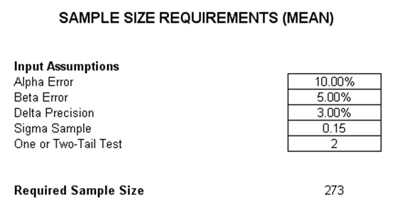
Figure 148.1: Sample size determination model for the mean
The remaining models are very similar in that they determine the appropriate sample size to test the standard deviation or sigma levels given some Alpha and Beta levels (Six Sigma – Sample Size Sigma), testing proportions (Six Sigma – Sample Size Proportion), or defect per unit (Six Sigma – Sample Size DPU). In addition, the Six Sigma – Sample Size Correlation model is used to determine the minimum required sample size to perform a hypothesis test on correlations. Finally, the Six Sigma – Delta Precision model works backwards in that given some Alpha and Beta errors and a given sample size, the Delta precision level is computed instead.
Design of Experiments (DOE) and Combinatorics
Another issue related to sampling and testing or experimentation is that of generating the relevant combinations and permutations of experimental samples to test. Let us say you have five different projects and need to decide all the combinations of projects that can occur. For instance, the value 00000 means no projects are chosen; or 10000, where project 1 is chosen and no others; or 010000 where project 2 is chosen and no others; and so forth. This result can also include multiple projects such as 10101 where projects 1, 3, and 5 are chosen. Clearly, if the portfolio has more projects, the combinations can become rather intractable. This is where combinatorial math comes in. We use Excel to determine the combinatorials.
Procedure
- Start Excel’s Analysis Toolpak (Tools | Add-Ins | Analysis Toolpak).
- Go to the Combinatorics modeland view the examples.
The example shown illustrates how to convert a five-project or five-asset portfolio into all the possible combinations by using the DEC2BIN function in Excel. The DEC2BIN function stands for decimal to binary function. Specifically, it takes the value of a decimal or number and converts it into the relevant binary structure of 0s and 1s.
For instance, if there are five projects in a portfolio, then there are 32 combinations or 25 combinations. As binary coding starts from 0, we can number these outcomes from 0, 1, 2, all the way to 31 (providing 32 possible outcomes). We then convert these to a five-digit binary sequence using the function DEC2BIN(0,5), which yields 00000. As another example, DEC2BIN(10,5) yields 01010, and so forth. By creating this combinatorial matrix, we see all the possible combinations for five projects. We can then pick out the ones required. For example, say we need to select two out of five projects, and need all the possible combinations. We know that there are 10 combinations, and by using the example model, we can determine exactly what they are. Figure 148.2 shows an example.
Using this approach, we can add in Risk Simulator to randomly select the projects and cycle through all possible combinations of projects that can be executed in time. As an example, say you have five projects in a portfolio and you would like to randomly choose three projects to execute in a sequence of three years. In each year you cannot execute more than three projects, and no project can repeat itself. In addition, you wish to run all possible combinations of possibilities. Such an example is also included in the model and is self-explanatory.
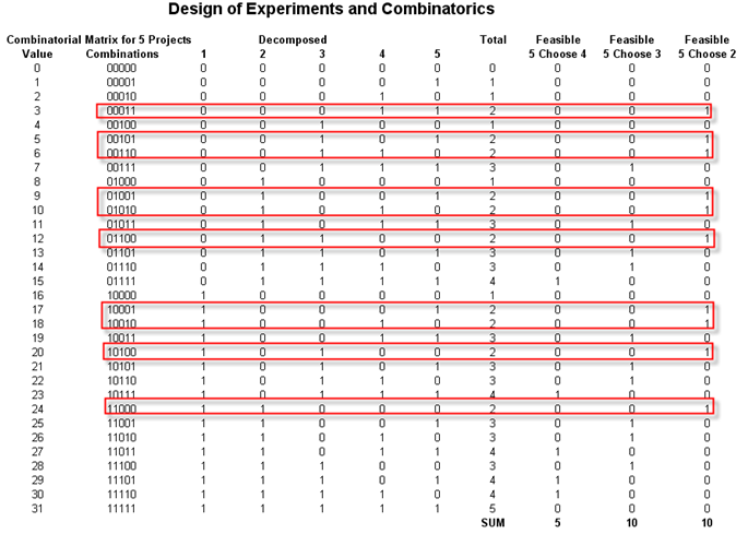
Figure 148.2: Combinatorics results