Theory
The J-curve, or exponential growth curve, is one where the growth of the next period depends on the current period’s level and the increase is exponential. This phenomenon means that over time, the values will increase significantly, from one period to another. This model is typically used in forecasting biological growth and chemical reactions over time.
Procedure
- Start Excel and select Risk Simulator | Forecasting | JS Curves.
- Select the J- or S-curve type, enter the required input assumptions (see Figures 11.16 and 11.17 for examples), and click OK to run the model and report.
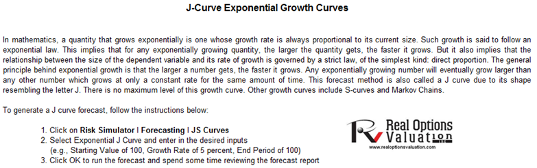
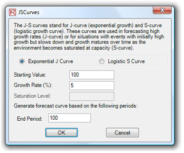
Figure 11.16: J-curve Forecast
The S-curve, or logistic growth curve, starts off like a J-curve, with exponential growth rates. Over time, the environment becomes saturated (e.g., market saturation, competition, overcrowding), the growth slows, and the forecast value eventually ends up at a saturation or maximum level. The S-curve model is typically used in forecasting market share or sales growth of a new product from market introduction until maturity and decline, population dynamics, growth of bacterial cultures, and other naturally occurring variables. Figure 11.17 illustrates a sample S-curve.
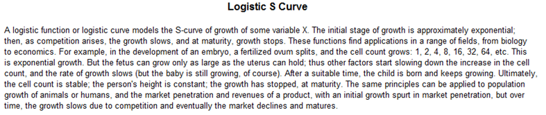
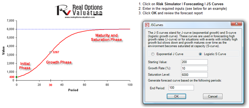
Figure 11.17: S-curve Forecast