File Name: Simulation – Basic Simulation Model
Location: Modeling Toolkit | Risk Simulator | Basic Simulation Model
Brief Description: Illustrates how to use Risk Simulator for running a Monte Carlo simulation, viewing and interpreting forecast results, setting seed values, setting run preferences, extracting simulation data, and creating new and switching among simulation profiles
Requirements: Modeling Toolkit, Risk Simulator
The model in the Static and Dynamic Model worksheet illustrates a very simple model with two input assumptions (revenue and cost) and an output forecast (income). In Figure 132.1, the model on the left is a static model with single-point estimates; the model on the right is a dynamic model on which Monte Carlo assumptions and forecasts can be created. After running the simulation, the results can be extracted and further analyzed. In this model, we can also learn to set different simulation preferences, run a simulation with error and precision controls, and set seed values. This should be the first model you run to get started with Monte Carlo simulation.
Figure 132.1 shows this basic model, which is a very simplistic model of revenue minus cost to equal income. On the static model, the input and output values are unchanging or static. This means that if revenue is $2 and the cost is $1, then the income must be $2 – $1, or $1. We replicate the same model on the right and call it a dynamic model, where we will run a simulation.
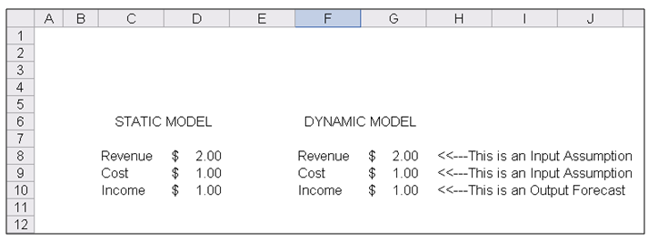
Figure 132.1: The world’s simplest model
Running a Monte Carlo Simulation
To run this model, simply:
- Select Risk Simulator | New Simulation Profile (or click on the New Profile icon in Figure 132.2) and provide it with a name.
- Select cell G8 and click on Risk Simulator | Set Input Assumption (or click on the Set Input Assumption icon shown in Figure 132.2).
- Select Triangular Distribution and set the Min = 1.50, Most Likely = 2.00, and Max = 2.25 and hit OK (Figure 132.3).
- Select cell G9 and set another input This time use Uniform Distribution with Min = 0.85 and Max = 1.25.
- Select cell G10 and set that cell as the output forecast by clicking on Risk Simulator | Set Output Forecast.
- Select Risk Simulator | Run Simulation (or click on the RUN icon in Figure 132.2) to start the simulation.
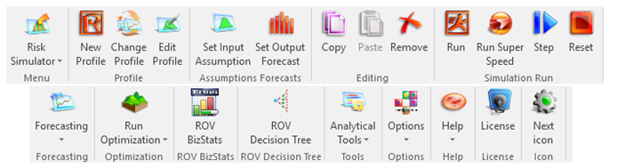
Figure 132.2: Risk Simulator toolbar
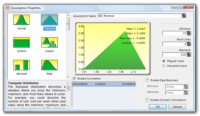
Figure 132.3: Setting up an assumption
Viewing and Interpreting Forecast Results
The forecast chart is shown when the simulation is running. Once simulation is completed, the forecast chart can be used (Figure 132.4). The forecast chart has several tabs, including Histogram, Statistics, Preferences, and Options tabs. Of particular interest are the first two tabs. For instance, the Histogram shows the output forecast’s probability distribution in the form of a histogram, where the specific values can be determined using the certainty boxes. For example, select Two-Tail, enter 90 in the certainty box, and hit TAB on the keyboard. The 90% confidence interval is shown (0.5273 and 1.1739), meaning that there is a 5% chance that the income will fall below $0.5273 and another 5% chance that it will be above $1.1739. Alternatively, you can select Left-Tail and enter 1.0 on the input box, hit TAB, and see that the left-tail certainty is 74.30%, indicating that there is a 74.30% chance that the income will fall below $1.0 (alternatively, there is a 25.70% chance that income will exceed $1.0).
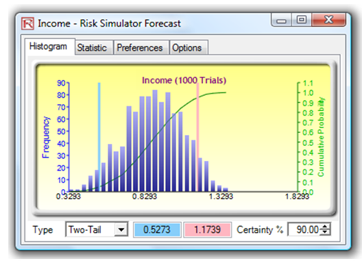
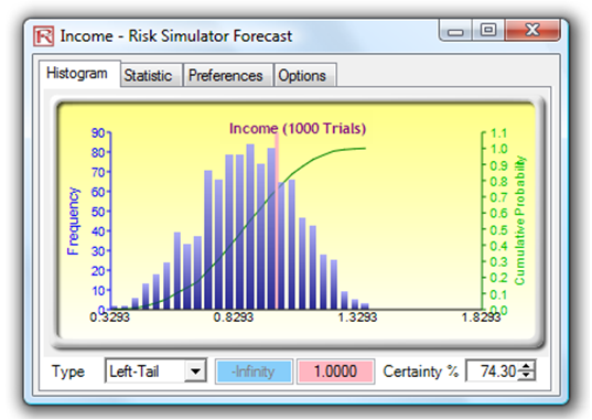
Figure 132.4: Forecast charts
The Statistics tab (Figure 132.5) illustrates the statistical results of the forecast variable. Note that your results will not be exactly the same as those illustrated here because a simulation (random number generation) was run. By definition, the results will not be exactly the same every time. However, if a seed value is set (see next section), the results will be identical in every single run. Setting a seed value is important especially when you wish to obtain the same values in each simulation run (e.g., you need the live model to return the same results as a printed report during a presentation).
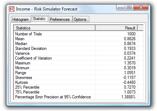
Figure 132.5: Statistics tab
Setting a Seed Value
- Reset the simulation by selecting Risk Simulator | Reset Simulation.
- Select Risk Simulator | Edit Simulation Profile.
- Select the check box for random number sequence.
- Enter in a seed value(e.g., 999) and hit OK (Figure 132.6).
- Run the simulation and note the results, then rerun the simulation a few times and verify that the results are the same as those obtained earlier.
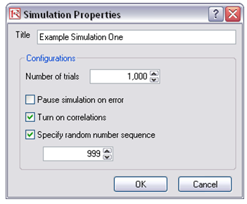
Figure 132.6: Setting a random number sequence seed
Note that the random number sequence or seed number has to be a positive integer value. Running the same model with the same assumptions and forecasts with the identical seed value and the same number of trials will always yield the same results. The number of simulation trials to run can be set in the same run properties box.
Setting Run Preferences
The run preferences dialog box allows you to specify the number of trials to run in a particular simulation. In addition, the simulation can be paused if a computational error in Excel is encountered (e.g., #NUM or #ERROR). Correlations can also be specified between pairs of input assumptions (Figure 132.3), and if Turn on Correlations is selected, these specified correlations will be imputed in the simulation.
Extracting Simulation Data
The simulation’s assumptions and forecast data are stored in memory until the simulation is reset or when Excel is closed. If required, these raw data can be extracted into a separate Excel spreadsheet. To extract the data, simply:
- Run the simulation.
- After the simulation is completed, select Risk Simulator | Analytical Tools | Extract Data.
- Choose the relevant assumptions or forecasts to extract and click OK (Figure 132.7).
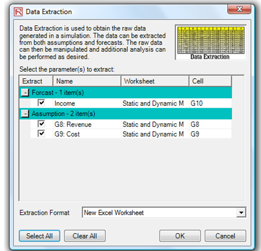
Figure 132.7: Data extraction
Creating New and Switching Among Simulation Profiles
The same model can have multiple simulation profiles in Risk Simulator. That is, different users of the same model can create their own simulation assumptions, forecasts, run preferences, and so forth. All these preferences are stored in separate simulation profiles, and each profile can be run independently. This powerful feature allows multiple users to run the same model their own way or allows the same user to run the model under different simulation conditions, thereby allowing for scenario analysis on Monte Carlo simulation. To create different profiles and switch among different profiles, simply:
- Create several new profiles by clicking on Risk Simulator | New Simulation Profile.
- Add the relevant assumptions and forecasts, or change the run preferences as desired in each simulation profile.
- Switch among different profiles by clicking on Risk Simulator | Change Active Simulation (Figure 132.8).
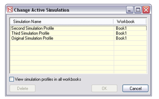
Figure 132.8: Switching among profiles