File Name: Options Analysis – Options Strategies
Location: Modeling Toolkit | Options Analysis | Options Trading Strategies
Brief Description: Illustrates various options trading strategies such as covered calls, protective puts, bull and bear spreads, straddles, and strangles
Requirements: Modeling Toolkit
Modeling Toolkit Functions Used: MTOptionStrategyLongCoveredCall, MTOptionStrategyWriteCoveredCall, MTOptionStrategyLongProtectivePut, MTOptionStrategyWriteProtectivePut, MTOptionStrategyLongBullDebitSpread, MTOptionStrategyLongBearDebitSpread, MTOptionStrategyLongBullCreditSpread, MTOptionStrategyLongBearCreditSpread, MTOptionStrategyLongStraddle, MTOptionStrategyWriteStraddle, MTOptionStrategyLongStrangle, MTOptionStrategyWriteStrangle
We start by discussing a simple option example. Suppose ABC’s stock is currently trading at $100, you can either purchase 1 share of ABC stock or purchase an options contract on ABC. Let’s see what happens. If you purchase the stock at $100 and in 3 months the stock goes up to $110, you made $10 or 10%. And if it goes down to $90, you lost $10 or 10%. This is simple enough. Now, suppose you purchased a European call option with a strike price of $100 (at the money) for a 3-month expiration that cost $5. If the underlying stock price goes up to $110, you execute the call option, buy the stock at $100 contractually, and sell the stock in the market at $110; after the cost of the option, you net $110 – $100 – $5 = $5. The cost of the option was $5, and you made $5, so the return was 100%. If the stock goes down to $90, you let the option expire worthless and lose the $5 payment to buy the option, rather than lose $10 if you held the stock. In addition, if the stock goes to $0, you only lose $5 if you held the option versus losing $100 if you held the stock! This shows the limited downside of the option and unlimited upside leverage, the concept of hedging. The problem is you can purchase many options through the leverage power of options. For instance, if you buy 20 options at $5 each, it costs you $100, the same as holding one stock. If the stock stays at $100 at maturity, you lose nothing on the stock, but you would lose 100% of your option premium. This is the concept of speculation!
Now, let’s complicate things. We can represent the payoffs on call and put options graphically as seen in Figure 107.1. For instance, take the call option with a strike price of $10 purchased when the stock price was also $10. The premium paid to buy the option was $2. Therefore, if at maturity the stock price goes up to $15, the call option is executed (buy the stock at the contractual price of $10, turn around and sell the stock at the market price of $15, make $5 in gross profits, and deducting the cost of the option of $2 yields a net profit of $3). Following the same logic, the remaining payoff schedule can be determined as shown in Figure 107.1. Note that the break-even point is when the stock price is $12 (strike price plus the option premium). If the stock price falls to $10 or below, the net is –$2 (loss) because the option will never be exercised, and the loss is the premium paid on the option. We can now chart the payoff schedules for buying (long) and selling (short) simple calls and puts. The “hockey stick” charts shown in Figure 107.1 are the various option payoff schedules.
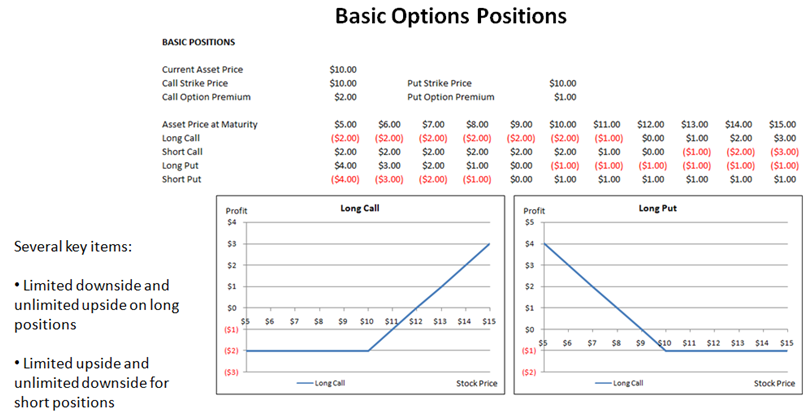
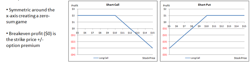 Figure 107.1: Basic option payoff schedule
Next, we can use these simple calls and puts and put them in a portfolio or in various combinations to create options trading strategies. Options trading strategy refers to the use of multiple investment vehicles, including call options, put options, and the underlying stock. These vehicles can be purchased or sold at various strike prices to create strategies that will take advantage of certain market conditions. For instance, Figure 107.2 shows a Covered Call strategy, which comprises a long stock and short call combination. The position requires buying a stock and simultaneously selling a call option on that stock. The colored charts in the Excel model provide a better visual than those shown in this chapter. Please refer to the model for more details.
Just as in previous chapters, the functions used are matrices, where the first row is always the stock price at maturity, the second and third rows are the individual positions’ net returns (e.g., in the case of the covered call, the second row represents the returns on the stock and the third row represents the short call position), and the fourth row is always the net total profit of the positions combined. As usual, apply the relevant Modeling Toolkit equations, copy and paste the cell’s functions to a matrix comprising 4 rows by 18 columns, select the entire matrix area, hold down the Shift + Control keys, and hit Enter to fill in the entire matrix. There are also two optional input parameters, the starting and ending points on the plot. These values refer to the starting and ending stock prices at maturity to analyze. If left empty, the software will automatically decide on these values.
The model also illustrates other options trading strategies. Figures 107.3 and 107.4 show the graphical representation of these positions, and the following lists these strategies and how they are obtained.
- A long covered call position is a combination of buying the stock (underlying asset) and selling a call of the same asset, typically at a different strike price than the starting stock price.
- A covered call is a combination of selling the stock (underlying asset) and buying a call of the same asset, typically at a different strike price than the starting stock price.
- A long protective put position is a combination of buying the stock (underlying asset) and buying a put of the same asset, typically at a different strike price than the starting stock price.
- Writing a protective put is a combination of selling the stock (underlying asset) and selling a put of the same asset, typically at a different strike price than the starting stock price.
- A long bull spread position is the same as writing a bearish spread, both of which are designed to be profitable if the underlying security rises in price. A bullish debit spread involves purchasing a call and selling a further out-of-the-money call. A bullish credit spread involves selling a put and buying a further out-of-the-money put.
- A long bearish spread takes advantage of a falling market, and the strategy involves the simultaneous purchase and sale of options; both puts and calls can be used. Typically, a higher strike price option is purchased, and a lower strike price option is sold. The options should have the same expiration date.
- A long bull spread position is the same as writing a bearish spread, both of which are designed to be profitable if the underlying security rises in price. A bullish debit spread involves purchasing a call and selling a further out-of-the-money call. A bullish credit spread involves selling a put and buying a further out-of-the money put.
- A long bearish spread takes advantage of a falling market, and the strategy involves the simultaneous purchase and sale of options; both puts and calls can be used. Typically, a higher strike price is purchased, and a lower strike price is sold. The options should have the same expiration date.
- A long straddle position requires the purchase of an equal number of puts and calls with identical strike price and expiration. A straddle provides the opportunity to profit from a prediction about the future volatility of the market. Long straddles are used to profit from high volatility, but the direction of the move is unknown.
- Writing a straddle position requires the sale of an equal number of puts and calls with identical strike price and expiration. A straddle provides the opportunity to profit from a prediction about the future volatility of the market. Writing a straddle is used to profit from low volatility, but the direction of the move is unknown.
- A long strangle requires the purchase of an out-of-the-money call and the purchase of an out-of-the-money put for a similar expiration (or within the same month), and profits from significant volatility of either directional move of the stock.
- Writing a strangle strategy requires the sale of an out-of-the-money call and the sale of an out-of-the-money put for a similar expiration (or within the same month) and profits from low volatility of either directional move of the stock.
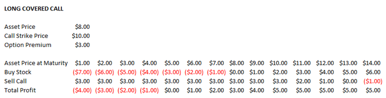
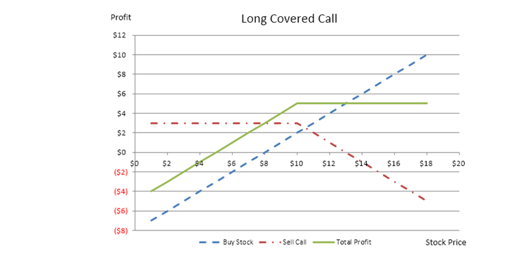
Figure 107.2: Covered call payoff schedule
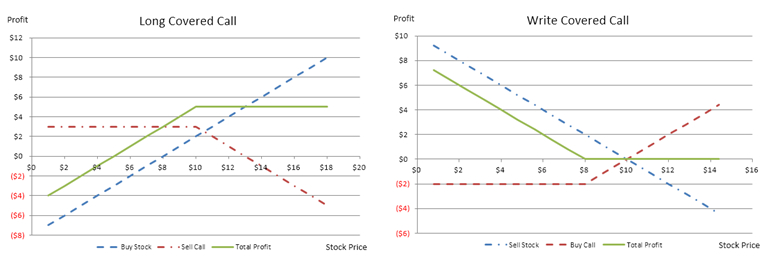
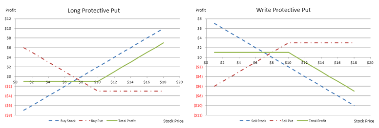
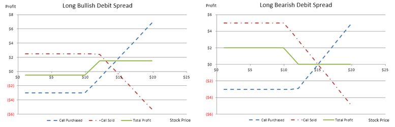
Figure 107.3: Options trading payoff schedule I
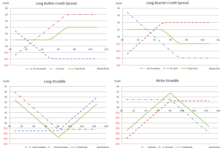
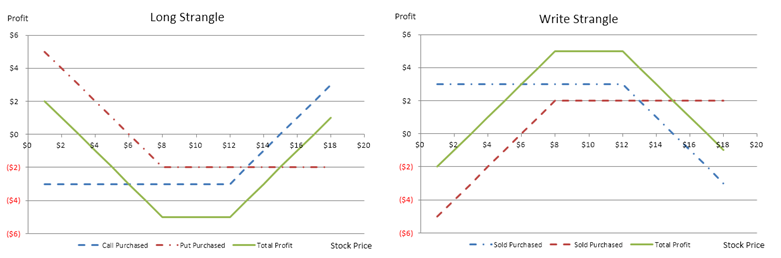
Figure 107.4: Options trading payoff schedule II