File Name: Forecasting – Stochastic Processes and others
Location: Modeling Toolkit | Forecasting | Stochastic Processes, as well as various models such as the Brownian Motion, Jump Diffusion, Forecast Distribution at Horizon, and Mean Reverting Stochastic Processes
Brief Description: Illustrates how to simulate Stochastic Processes (Brownian Motion Random Walk, Mean-Reversion, Jump-Diffusion, and Mixed Models)
Requirements: Modeling Toolkit, Risk Simulator
A stochastic process is a sequence of events or paths generated by probabilistic laws. That is, random events can occur over time but are governed by specific statistical and probabilistic rules. The main stochastic processes include Random Walk or Brownian Motion, Mean-Reversion, and Jump-Diffusion. These processes can be used to forecast a multitude of variables that seemingly follow random trends but yet are restricted by probabilistic laws. We can use Risk Simulator’s Stochastic Process module to simulate and create such processes. These processes can be used to forecast a multitude of time-series data including stock prices, interest rates, inflation rates, oil prices, electricity prices, commodity prices, and so forth.
Stochastic Process Forecasting
To run this model, simply:
- Select Risk Simulator | Forecasting | Stochastic Processes.
- Enter a set of relevant inputs or use the existing inputs as a test case (Figure 89.1).
- Select the relevant process to simulate.
- Click on Update Chart to view the updated computation of a single path or click OK to create the process.
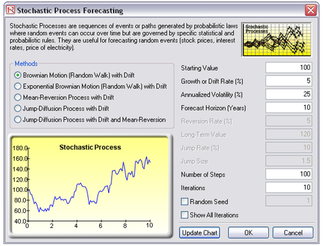
Figure 89.1: Running a stochastic process forecast
Model Results Analysis
For your convenience, the analysis Report worksheet is included in the model. A stochastic time-series chart and forecast values are provided in the report as well as each step’s time period, mean, and standard deviation of the forecast (Figure 89.2). The mean values can be used as the single-point estimate, or assumptions can be manually generated for the desired time period. That is, after finding the appropriate time period, create an assumption with a normal distribution with the appropriate mean and standard deviation computed. A sample chart with 10 iteration paths is included to graphically illustrate the behavior of the forecasted process.
Clearly, the key is to calibrate the inputs to a stochastic process forecast model. The input parameters can be obtained very easily through some econometric modeling of historical data. The Data Diagnostic and Statistical Analysis models show how to use Risk Simulator to compute these input parameters. See Dr. Johnathan Mun’s Modeling Risk, Third Edition (Thomson–Shore, 2015), for the technical details on obtaining these parameters.
The Risk Simulator tool is useful for quickly generating large numbers of stochastic process forecasts. Alternatively, if the inputs are uncertain and need to be simulated, use Modeling Toolkit’s examples, Brownian Motion Stochastic Process, Jump Diffusion Stochastic Process, or Mean Reverting Stochastic Process models (all of these are located in the Modeling Toolkit | Forecasting menu item). Finally, a deterministic model on stock price forecast assuming a random walk process is also available (Modeling Toolkit | Forecasting | Forecast Distribution) where the stock price forecasts are provided for a future date.
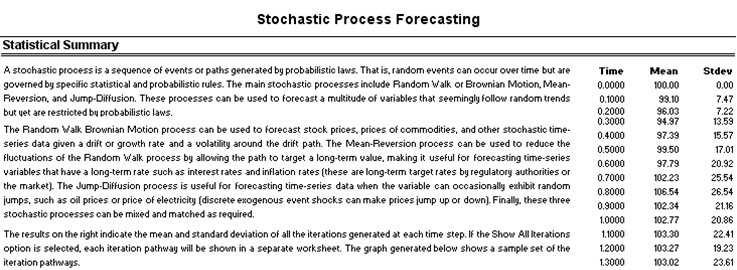
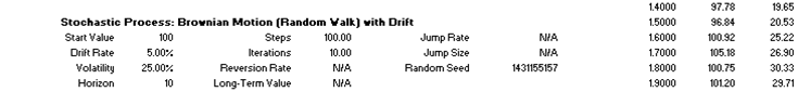
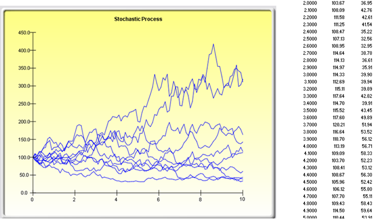
Figure 89.2: Stochastic process forecast results