This sample model illustrates how to use Risk Simulator for:
- Running Static, Dynamic, and Stochastic Optimization with Continuous Decision Variables
- Optimization with Discrete Integer Decision Variables
- Efficient Frontier and Advanced Optimization Settings
Model Background
1. Running Static, Dynamic, and Stochastic Optimization with Continuous Decision Variables
Figure 17E.A illustrates the continuous optimization example model. In this example, there are 10 distinct asset classes (e.g., different types of mutual funds, stocks, or assets) where the idea is to most efficiently and effectively allocate the portfolio holdings such that the best bang for the buck is obtained. In other words, we want to generate the best portfolio returns possible given the risks inherent in each asset class. In order to truly understand the concept of optimization, we will have to delve more deeply into this sample model to see how the optimization process can best be applied. The model shows the 10 asset classes and each asset class has its own set of annualized returns and annualized volatilities. These return and risk measures are annualized values such that they can be consistently compared across different asset classes. Returns are computed using the geometric average of the relative returns, while the risks are computed using the logarithmic relative stock returns approach.
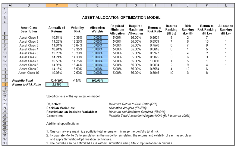
Figure 17E.A: Continuous Optimization Model
The Allocation Weights in column E holds the decision variables, which are the variables that need to be tweaked and tested such that the total weight is constrained at 100% (cell E17). Typically, to start the optimization, we will set these cells to a uniform value, where in this case, cells E6 to E15 are set at 10% each. In addition, each decision variable may have specific restrictions in its allowed range. In this example, the lower and upper allocations allowed are 5% and 35%, as seen in columns F and G. This means that each asset class may have its own allocation boundaries. Next, column H shows the return to risk ratio, which is simply the return percentage divided by the risk percentage; the higher this value, the higher the bang for the buck. The remaining columns show the individual asset class rankings by returns, risk, return to risk ratio, and allocation. In other words, these rankings show at a glance which asset class has the lowest risk or the highest return, and so forth. The portfolio’s total returns in cell C17 is SUMPRODUCT(C6:C15, E6:E15), that is, the sum of the allocation weights multiplied by the annualized returns for each asset class. In other words, we have ![]() where RP is the return on the portfolio, RA,B,C,D are the individual returns on the projects, and ωA,B,C,D are the respective weights or capital allocation across each project. In addition, the portfolio’s diversified risk in cell D17 is computed by taking
where RP is the return on the portfolio, RA,B,C,D are the individual returns on the projects, and ωA,B,C,D are the respective weights or capital allocation across each project. In addition, the portfolio’s diversified risk in cell D17 is computed by taking![]()
Here, ρi,j are the respective cross-correlations between the asset classes—hence, if the cross-correlations are negative, there are risk diversification effects, and the portfolio risk decreases. However, to simplify the computations here, we assume zero correlations among the asset classes through this portfolio risk computation but assume the correlations when applying simulation on the returns as will be seen later. Therefore, instead of applying static correlations among these different asset returns, we apply the correlations in the simulation assumptions themselves, creating a more dynamic relationship among the simulated return values. Finally, the return to risk ratio or Sharpe Ratio is computed for the portfolio. This value is seen in cell C18 and represents the objective to be maximized in this optimization exercise.
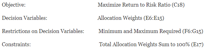
The following are the specifications in this example optimization model:
Procedure
- Start Excel and open the example file Risk Simulator | Example Models | 11 Optimization Continuous.
- Start a new profile with Risk Simulator | New Profile (or click on the New Profile icon) and give it a name.
- The first step in optimization is to set the decision variables. Select cell E6 and set the first decision variable (Risk Simulator | Optimization | Set Decision) or click on the D Then click on the link icon to select the name cell (B6), as well as the lower bound and upper bound values at cells F6 and G6. Then, using Risk Simulator Copy, copy this cell E6 decision variable and paste the decision variable to the remaining cells in E7 to E15.
- The second step in optimization is to set the constraint. There is only one constraint here, that is, the total allocation in the portfolio must sum to 100%. So, click on Risk Simulator | Optimization | Constraints… or click on the C icon, and select ADD to add a new constraint. Then, select cell E17 and make it equal (=) to 100%. Click OK when done.
- Exercise Question: Would you get the same results if you set E7 = 1 instead of 100%?
- Exercise Question: In the constraints user interface, what does the Efficient Frontier button mean, and how does it work?
- The final step in optimization is to set the objective function. Select cell C18 and click on Risk Simulator | Optimization | Set Objective or click on the O icon. Check to make sure the objective cell is set for C18 and select Maximize.
- Start the optimization by going to Risk Simulator | Optimization | Run Optimization or click on the Run Optimization icon and select the optimization of choice (Static Optimization, Dynamic Optimization, or Stochastic Optimization). To get started, select Static Optimization. You can now review the objective, decision variables, and constraints in each tab if required, or click OK to run the static optimization.
- Exercise Question: In the Run Optimization user interface, click on the Statistics tab and you see that there is nothing there. Why?
- Once the optimization is complete, you may select Revert to revert back to the original values of the decision variables as well as the objective, or select Replace to apply the optimized decision variables. Typically, Replace is chosen after the optimization is done. Then review the Results Interpretation section below before proceeding to the next step in the exercise.
- Now reset the decision variables by typing 10% back into all cells from E6 to E15. Then, select cell C6 and Risk Simulator | Set Input Assumption and use the default Normal distribution and the default parameters. This is only an example run and we really do not need to spend time to set proper distributions. Repeat setting the normal assumptions for cells C7 to C15.
- Exercise Question: Should you or should you not copy the first assumption in cell C6 and then copy and paste the parameters to cells C7:C15? And if we copy and paste the assumptions, what is the difference between using Risk Simulator Copy and Paste functions as opposed to using Excel’s copy and paste function? What happens when you first hit Escape before applying Risk Simulator Paste?
- Exercise Question: Why do we need to enter 10% back into the cells?
- Now run the optimization Risk Simulator | Optimization | Run Optimization and this time select Dynamic Optimization in the Method tab. When completed, click on Revert to go back to the original 10% decision variables.
- Exercise Question: What was the difference between the static optimization run in Step 6 above and dynamic optimization?
- Now run the optimization Risk Simulator | Optimization | Run Optimization a third time, but this time, select Stochastic Optimization in the Method tab. Then notice several things.
- First, click on the Statistics tab and see that this tab is now populated. Why is this the case and how do you use this statistics tab?
- Second, click on the Advanced button and select the checkbox Run Super Speed Simulation. Then click OK to run the optimization. What do you see? How is super speed integrated into stochastic optimization?
- Access the advanced options by going to Risk Simulator | Optimization | Run Optimization and clicking the Advanced button. Spend some time trying to understand what each element means and how it is pertinent to optimization.
- After running the stochastic optimization, a report is created. Spend some time reviewing the report and try to understand what it means, as well as review the forecast charts generated for each decision
Figure 17E.B shows the screenshots of the procedural steps given above. You can add simulation assumptions on the model’s returns and risk (columns C and D) and apply dynamic optimization and stochastic optimization for additional practice.
Results Interpretation
The optimization’s final results are shown in Figure 17E.C, where the optimal allocation of assets for the portfolio is seen in cells E6:E15. That is, given the restrictions of each asset fluctuating between 5% and 35%, and where the sum of the allocation must equal 100%, the allocation that maximizes the return to risk ratio is seen in Figure 17E.C. A few important things have to be noted when reviewing the results and optimization procedures performed thus far:
- The correct way to run the optimization is to maximize the bang for the buck or returns to risk Sharpe Ratio as we have done.
- If instead, we maximized the total portfolio returns, the optimal allocation result is trivial and does not require optimization to obtain. That is, simply allocate 5% (the minimum allowed) to the lowest 8 assets, 35% (the maximum allowed) to the highest returning asset, and the remaining (25%) to the second-best returns asset. Optimization is not required. However, when allocating the portfolio this way, the risk is a lot higher as compared to when maximizing the returns to risk ratio, although the portfolio returns by themselves are higher.
- Conversely, one can minimize the total portfolio risk, but the returns will be less.
The following table illustrates the results from the three different objectives being optimized:
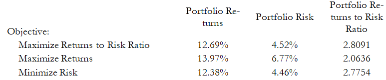
From the table, it can be seen that the best approach is to maximize the returns to risk ratio. That is, for the same amount of risk, this allocation provides the highest amount of return. Conversely, for the same amount of return, this allocation provides the lowest amount of risk possible. This approach of bang for the buck or returns to risk ratio is the cornerstone of the Markowitz efficient frontier in modern portfolio theory. That is, if we constrained the total portfolio risk level and successively increased it over time, we will obtain several efficient portfolio allocations for different risk characteristics. Thus, different efficient portfolio allocations can be obtained for different individuals with different risk preferences.
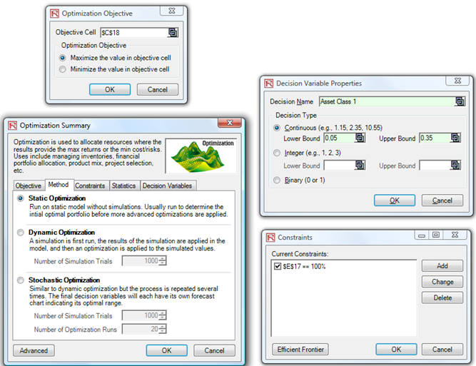
Figure 17E.B: Running Continuous Optimization in Risk Simulator
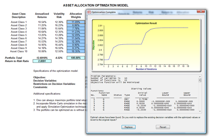
Figure 17E.C: Continuous Optimization Results
2. Optimization with Discrete Integer Decision Variables
Sometimes, the decision variables are not continuous but discrete integers (e.g., 1, 2, 3) or binary (e.g., 0 and 1). In the binary situation, we can use such optimization as on-off switches or go/no-go decisions. Figure 17E.D illustrates a project selection model where there are 12 projects listed. The example here uses the Risk Simulator | Example Models | 12 Optimization Discrete model. As before, each project has its own returns (ENPV and NPV for expanded net present value and net present value—the ENPV is simply the NPV plus any strategic real options values), costs of implementation, risks, and so forth. If required, this model can be modified to include required full-time equivalences (FTE) and other resources of various functions, and additional constraints can be set on these additional resources. The inputs into this model are typically linked from other spreadsheet models. For instance, each project will have its own discounted cash flow or returns on investment model. The application here is to maximize the portfolio’s Sharpe Ratio subject to some budget allocation. Many other versions of this model can be created, for instance, maximizing the portfolio returns, or minimizing the risks, or adding additional constraints where the total number of projects chosen cannot exceed 6, and so forth and so on. All of these items can be run using this existing model.
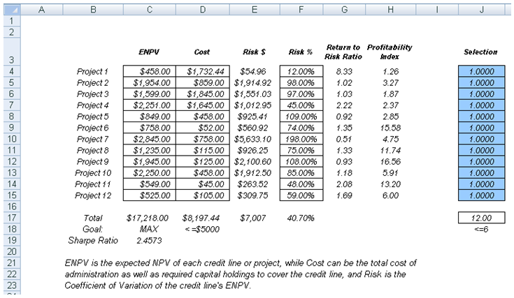
Figure 17E.D: Discrete Integer Optimization Model
Procedure
- Open the example file and start a new profile by clicking on Risk Simulator | New Profile and give it a name.
- The first step in optimization is to set up the decision variables. Set the first decision variable by selecting cell J4, and select Risk Simulator | Optimization | Set Decision or click on the D Then, click on the link icon to select the name cell (B4), and select the Binary Then, using Risk Simulator Copy, copy this cell J4 decision variable and paste the decision variable to the remaining cells in J5 to J15. This is the best method if you have only several decision variables and you can name each decision variable with a unique name for identification later.
- Exercise Question: What is the main purpose of linking the name to cell B4 before doing the copy and paste parameters?
- The second step in optimization is to set the constraint. There are two constraints here: The total budget allocation in the portfolio must be less than $5,000 and the total number of projects must not exceed 6. So, click on Risk Simulator | Optimization | Constraints… or click on the C icon and select ADD to add a new constraint. Then, select the cell D17 and make it D17 <= 5000. Repeat by setting cell J17 <= 6.
- Exercise Question: Why do we use <= instead of =?
- Exercise Question: Sometimes when there are no feasible results or the optimization does not run, changing the equal sign to the inequality helps. Why?
- Exercise Question: What would you do if you wanted D17 < 5000 instead of <= 5000?
- Exercise Question: Explain what would happen to the binding constraints if you set only one constraint and it is D17 <= 8200 or only J17 <= 12?
- The final step in optimization is to set the objective function and start the optimization by selecting cell C19 and selecting Risk Simulator | Optimization | Set Objective then, run the optimization using Risk Simulator | Optimization | Run Optimization and selecting the optimization of choice (Static Optimization, Dynamic Optimization, or Stochastic Optimization). To get started, select Static Optimization. Check to make sure that the objective cell is either the Sharpe Ratio or portfolio returns to risk ratio and select Maximize. You can now review the decision variables and constraints if required, or click OK to run the static optimization. Figure 17E.E shows the settings and Figure 17E.F shows a sample set of results of optimal selection of projects that maximizes the Sharpe Ratio.
- Exercise Question: If instead, you maximized total revenues by changing the existing objective, this becomes a trivial model and simply involves choosing the highest returning project and going down the list until you run out of money or exceed the budget constraint. Doing so will yield theoretically undesirable projects as the highest yielding projects typically hold higher risks. Do you agree? What other variables can be used as objective in this model, if any?
- Exercise Question: If we use the coefficient of variation instead of return to risk ratio, would we maximize or minimize this variable?
- Exercise Question: How would you model a situation where, say, one project is the prerequisite for another or if two or more projects are mutually exclusive? How do you model the following?
- You cannot do Project 2 by itself without Project 1, but you can do Project 1 on its own without Project 2.
- Either Project 3 or Project 4 can be chosen but not both.
- Each project has some full-time equivalence (FTE) employees required to be involved, and the company has a limited number of FTEs.
- Now add simulation assumptions on the model’s ENPV and cost variables (columns C and D) and apply dynamic optimization for additional practice.
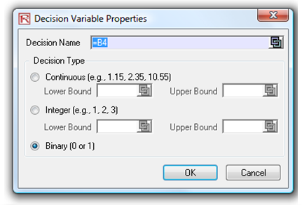
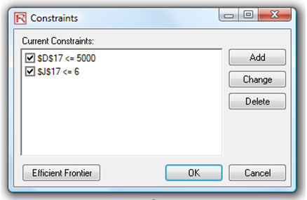
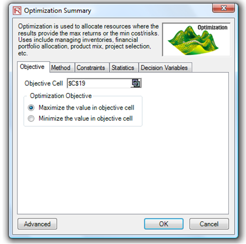
Figure 17E.E: Running Discrete Integer Optimization in Risk Simulator
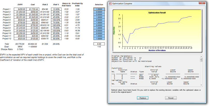
Figure 17E.F: Optimal Selection of Projects That Maximizes the Sharpe Ratio
3. Efficient Frontier and Advanced Optimization Settings
Figure 17E.G shows the Constraints for optimization. Here, if you clicked on the Efficient Frontier button after you have set some constraints, you can now make these constraints changing. That is, each of the constraints can be created to step through between some maximum and minimum value. As an example, the constraint in cell J17 <= 6 can be set to run between 4 and 8 (Figure 17E.G). That is, five optimizations will be run, each with the following constraints: J17 <= 4, J17 <= 5, J17 <= 6, J17 <= 7, and J17 <= 8. The optimal results will then be plotted as an efficient frontier and the report will be generated (Figure 17E.H). Specifically, the following illustrates the steps required to create a changing constraint:
- In an optimization model (i.e., a model with Objective, Decision Variables, and Constraints already set up), click on Risk Simulator | Optimization | Constraints and click on Efficient Frontier.
- Select the constraint you want to change or step, J17, and enter the parameters for Min, Max, and Step Size (Figure 17E.G). Then click ADD and then OK and OK again. Also, uncheck the first constraint of D17 <= 5000.
- Run Optimization as usual, Risk Simulator | Optimization | Run Optimization or click on the Run Optimization icon. You can choose static, dynamic, or stochastic when running an efficient frontier, but to get started, choose the static optimization routine.
- Exercise Question: What happens if you run a stochastic optimization with an efficient frontier? What is the step-by-step process that it goes through?
- Exercise Question: What happens if you do not uncheck the first constraint?
- The results will be shown as a user interface (Figure 17E.H). Click on Create Report to generate a report worksheet with all the details of the optimization runs.
- Exercise Question: How do you interpret the efficient frontier? Is a steeper curve better or a flatter curve? Can the curve slope downwards and if so, what does that mean?
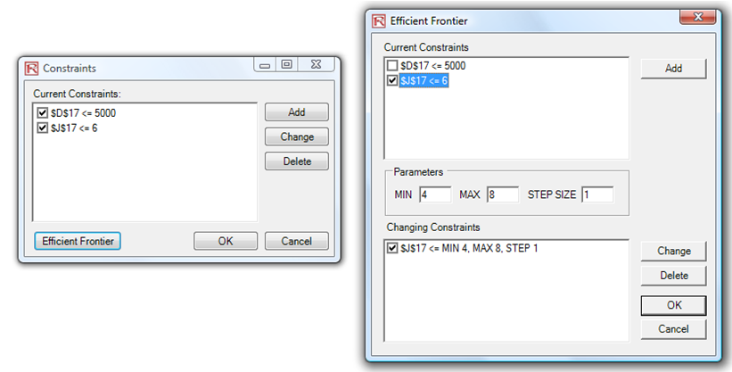
Figure 17E.G: Generating Changing Constraints in an Efficient Frontier
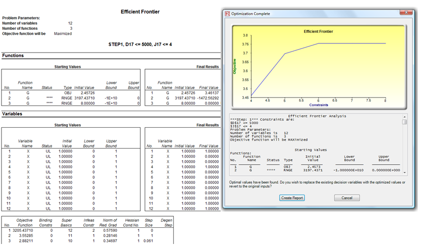
Figure 17E.H: Efficient Frontier Results