It is assumed that the user is sufficiently knowledgeable about the fundamentals of regression analysis. The general bivariate linear regression equation takes the form of ![]() where
where ![]() is the intercept,
is the intercept, ![]() is the slope, and ε is the error term. It is bivariate as there are only two variables, a Y or dependent variable, and an X or independent variable, where X is also known as the regressor (sometimes a bivariate regression is also known as a univariate regression as there is only a single independent variable X ). The dependent variable is named as such as it depends on the independent variable, for example, sales revenue depends on the amount of marketing costs expended on a product’s advertising and promotion, making the dependent variable sales and the independent variable marketing costs. An example of a bivariate regression is seen as simply inserting the best-fitting line through a set of data points in a two-dimensional plane, as seen on the left panel in Figure 9.38. In other cases, a multivariate regression can be performed, where there are multiple or k number of independent X variables or regressors, where the general regression equation will now take the form of
is the slope, and ε is the error term. It is bivariate as there are only two variables, a Y or dependent variable, and an X or independent variable, where X is also known as the regressor (sometimes a bivariate regression is also known as a univariate regression as there is only a single independent variable X ). The dependent variable is named as such as it depends on the independent variable, for example, sales revenue depends on the amount of marketing costs expended on a product’s advertising and promotion, making the dependent variable sales and the independent variable marketing costs. An example of a bivariate regression is seen as simply inserting the best-fitting line through a set of data points in a two-dimensional plane, as seen on the left panel in Figure 9.38. In other cases, a multivariate regression can be performed, where there are multiple or k number of independent X variables or regressors, where the general regression equation will now take the form of ![]() In this case, the best-fitting line will be within a k + 1 dimensional plane.
In this case, the best-fitting line will be within a k + 1 dimensional plane.
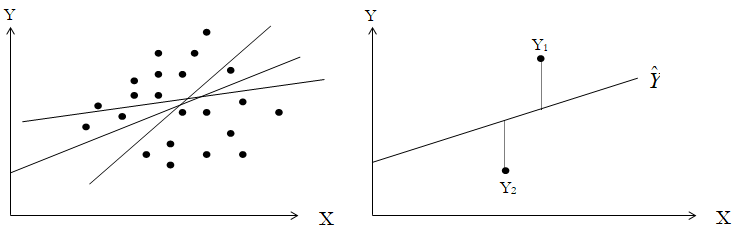
Figure 9.38: Bivariate Regression
However, fitting a line through a set of data points in a scatter plot as in Figure 9.38 may result in numerous possible lines. The best-fitting line is defined as the single unique line that minimizes the total vertical errors, that is, the sum of the absolute distances between the actual data points ![]() and the estimated line
and the estimated line ![]()
as shown on the right panel of Figure 9.38. To find the best-fitting unique line that minimizes the errors, a more sophisticated approach is applied, using regression analysis. Regression analysis finds the unique best-fitting line by requiring that the total errors be minimized, or by calculating
where only one unique line minimizes this sum of squared errors. The errors (vertical distances between the actual data and the predicted line) are squared to avoid the negative errors from canceling out the positive errors. Solving this minimization problem with respect to the slope and intercept requires calculating first derivatives and setting them equal to zero:
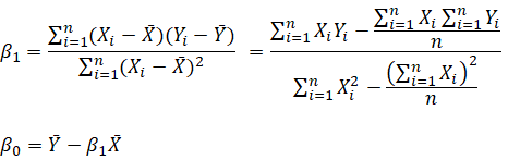
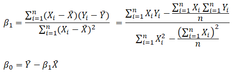
which yields the bivariate regression’s least squares equations:
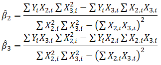
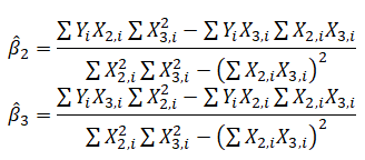
For multivariate regression, the analogy is expanded to account for multiple independent variables, where ![]() and the estimated slopes can be calculated by:
and the estimated slopes can be calculated by:
In running multivariate regressions, great care must be taken to set up and interpret the results. For instance, a good understanding of econometric modeling is required (e.g., identifying regression pitfalls such as structural breaks, multicollinearity, heteroskedasticity, autocorrelation, specification tests, nonlinearities, and so forth) before a proper model can be constructed.
Figure 9.39 shows how a multiple linear and nonlinear regression can be run in Risk Simulator. In Excel, type in or open your existing dataset (the illustration below uses Risk Simulator | Example Models | 09 Multiple Regression in the examples folder). Check to make sure that the data are arranged in columns and select the data including the variable headings and click on Risk Simulator | Forecasting| Multiple Regression. Select the dependent variable and check the relevant options (lags, stepwise regression, nonlinear regression, and so forth) and click OK. Figure 9.40 illustrates a sample multivariate regression result report generated. The report comes complete with all the regression results, analysis of variance results, fitted chart, and hypothesis test results.
See Chapter 12’s section on Regression Analysis for more technical details and manual computations of multiple regression methods.
![]()
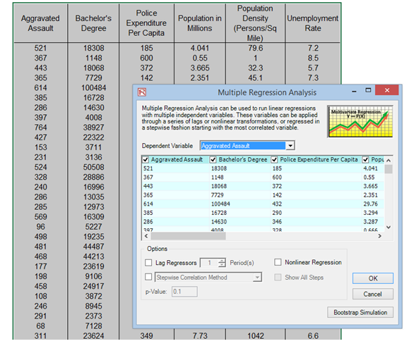
Figure 9.39: Regression in Risk Simulator
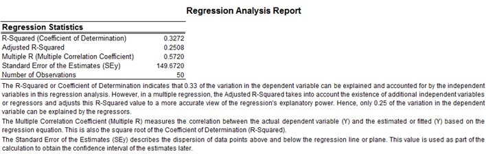
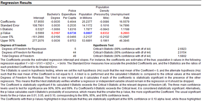
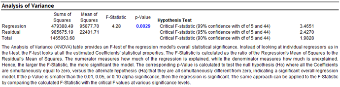
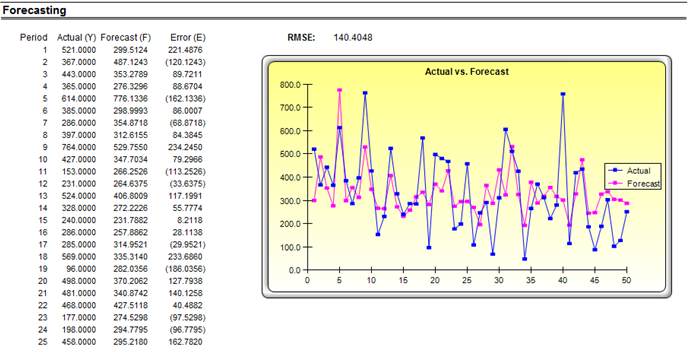
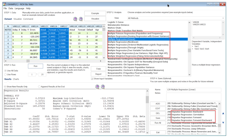
Figure 9.40: Regression Results in Risk Simulator & BizStats