Theory
The generalized autoregressive conditional heteroskedasticity (GARCH) model is used to model historical and forecast future volatility levels of a marketable security (e.g., stock prices, commodity prices, oil prices, etc.). The dataset has to be a time series of raw price levels. GARCH will first convert the prices into relative returns and then run an internal optimization to fit the historical data to a mean-reverting volatility term structure, while assuming that the volatility is heteroskedastic in nature (changes over time according to some econometric characteristics). The theoretical specifics of a GARCH model are outside the purview of this book.
Procedure
- Start Excel, open the example file Advanced Forecasting Model, go to the GARCH worksheet, and select Risk Simulator | Forecasting | GARCH.
- Click on the link icon, select the Data Location and enter the required input assumptions(see Figure 11.18), and click OK to run the model and report.
Notes
The typical volatility forecast situation requires P = 1, Q = 1; Periodicity = number of periods per year (12 for monthly data, 52 for weekly data, 252 or 365 for daily data); Base = minimum of 1 and up to the periodicity value; and Forecast Periods = number of annualized volatility forecasts you wish to obtain. There are several GARCH models available in Risk Simulator, including EGARCH, EGARCH-T, GARCH-M, GJR-GARCH, GJR-GARCH-T, IGARCH, and T-GARCH.
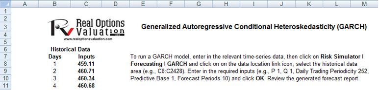
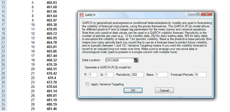
Figure 11.18: GARCH Volatility Forecast
GARCH models are used mainly in analyzing financial time-series data to ascertain their conditional variances and volatilities. These volatilities are then used to value the options as usual, but the amount of historical data necessary for a good volatility estimate remains significant. Usually, several dozen––and even up to hundreds––of data points are required to obtain good GARCH estimates. GARCH is a term that incorporates a family of models that can take on a variety of forms, known as GARCH(p,q), where p and q are positive integers that define the resulting GARCH model and its forecasts. In most cases for financial instruments, a GARCH(1,1) is sufficient and is most generally used. For instance, a GARCH (1,1) model takes the form of:
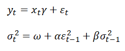
The first equation’s dependent variable![]() is a function of exogenous variables
is a function of exogenous variables![]() with an error term
with an error term![]() The second equation estimates the variance
The second equation estimates the variance![]() at time t, which depends on a historical mean (ω), news about volatility from the previous period, measured as a lag of the squared residuals from the mean equation
at time t, which depends on a historical mean (ω), news about volatility from the previous period, measured as a lag of the squared residuals from the mean equation![]() and volatility from the previous period
and volatility from the previous period![]() The exact modeling specification of a GARCH model is beyond the scope of this book. Suffice it to say that detailed knowledge of econometric modeling (model specification tests, structural breaks, and error estimation) is required to run a GARCH model, making it less accessible to the general analyst. Another problem with GARCH models is that the model usually does not provide a good statistical fit. That is, it is impossible to predict the stock market and, of course, equally if not harder to predict a stock’s volatility over time.
The exact modeling specification of a GARCH model is beyond the scope of this book. Suffice it to say that detailed knowledge of econometric modeling (model specification tests, structural breaks, and error estimation) is required to run a GARCH model, making it less accessible to the general analyst. Another problem with GARCH models is that the model usually does not provide a good statistical fit. That is, it is impossible to predict the stock market and, of course, equally if not harder to predict a stock’s volatility over time.
Note that the GARCH function has several inputs as follow:
- Time-Series Data. The time series of data in chronological order (e.g., stock prices). Typically, dozens of data points are required for a decent volatility forecast.
- Periodicity, A positive integer indicating the number of periods per year (e.g., 12 for monthly data, 252 for daily trading data, etc.), assuming you wish to annualize the volatility. To obtain periodic volatility, enter 1.
- Predictive Base. The number of periods back (of the time-series data) to use as a base to forecast volatility. The higher this number, the longer the historical base is used to forecast future volatility.
- Forecast Period. A positive integer indicating how many future periods beyond the historical stock prices you wish to forecast.
- Variance Targeting. This variable is set as False by default(even if you do not enter anything here) but can be set as True. False means the omega variable is automatically optimized and computed. The suggestion is to leave this variable empty. If you wish to create mean-reverting volatility with variance targeting, set this variable as True.
- P The number of previous lags on the mean equation.
- Q The number of previous lags on the variance equation.
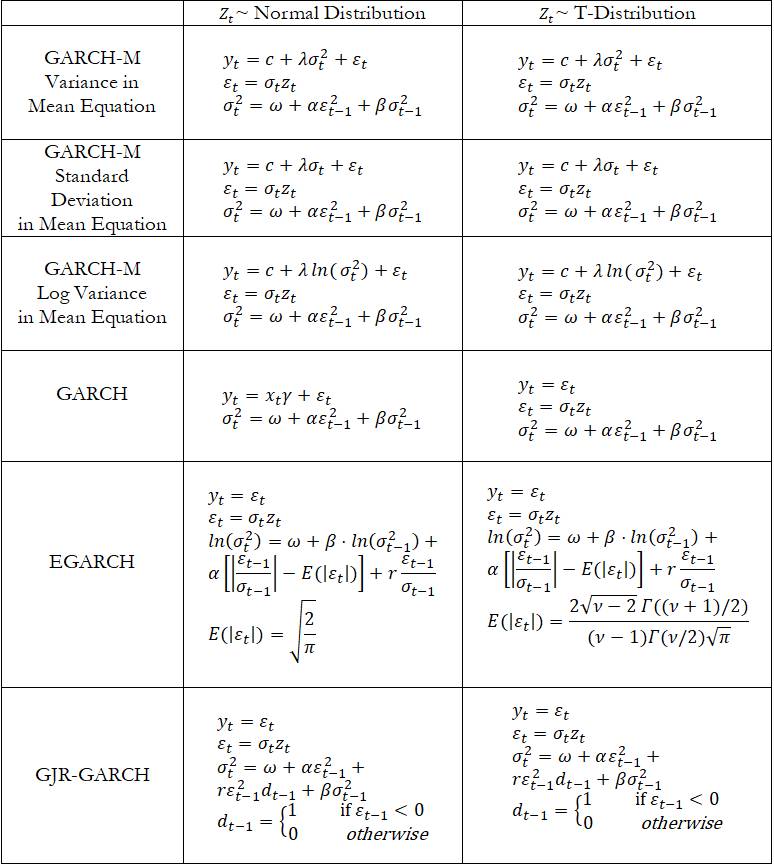
The accompanying chart shows some of the GARCH specifications used in Risk Simulator with two underlying distributional assumptions: one for normal distribution and the other for the t-distribution.
For the GARCH-M models, the conditional variance equations are the same in the six variations but the mean questions are different and assumptions on ![]() can be either normal distribution or t-distribution. The estimated parameters for GARCH-M with normal distribution are those five parameters in the mean and conditional variance equations. The estimated parameters for GARCH-M with the t-distribution are those five parameters in the mean and conditional variance equations plus another parameter, the degrees of freedom for the t-distribution. In contrast, for the GJR models, the mean equations are the same in the six variations and the differences are that the conditional variance equations and the assumption on can be either a normal distribution or t-distribution. The estimated parameters for EGARCH and GJR-GARCH with normal distribution are those four parameters in the conditional variance equation. The estimated parameters for GARCH, EGARCH, and GJR-GARCH with t-distribution are those parameters in the conditional variance equation plus the degrees of freedom for the t-distribution. More technical details of GARCH methodologies fall outside of the scope of this book.
can be either normal distribution or t-distribution. The estimated parameters for GARCH-M with normal distribution are those five parameters in the mean and conditional variance equations. The estimated parameters for GARCH-M with the t-distribution are those five parameters in the mean and conditional variance equations plus another parameter, the degrees of freedom for the t-distribution. In contrast, for the GJR models, the mean equations are the same in the six variations and the differences are that the conditional variance equations and the assumption on can be either a normal distribution or t-distribution. The estimated parameters for EGARCH and GJR-GARCH with normal distribution are those four parameters in the conditional variance equation. The estimated parameters for GARCH, EGARCH, and GJR-GARCH with t-distribution are those parameters in the conditional variance equation plus the degrees of freedom for the t-distribution. More technical details of GARCH methodologies fall outside of the scope of this book.