Theory
Limited Dependent Variables describe the situation where the dependent variable contains data that are limited in scope and range, such as binary responses (0 or 1), truncated, ordered, or censored data. For instance, given a set of independent variables (e.g., age, income, education level of credit card or mortgage loan holders), we can model the probability of defaulting on mortgage payments, using maximum likelihood estimation (MLE). The response or dependent variable Y is binary, that is, it can have only two possible outcomes that we denote as 1 and 0 (e.g., Y may represent presence/absence of a certain condition, defaulted/not defaulted on previous loans, success/failure of some device, answer yes/no on a survey, etc.) and we also have a vector of independent variable regressors X, which are assumed to influence the outcome Y. A typical ordinary least squares regression approach is invalid because the regression errors are heteroskedastic and non-normal, and the resulting estimated probability estimates will return nonsensical values of above 1 or below 0. MLE analysis handles these problems using an iterative optimization routine to maximize a log-likelihood function when the dependent variables are limited.
A Logit or Logistic regression is used for predicting the probability of occurrence of an event by fitting data to a logistic curve. It is a generalized linear model used for binomial regression, and like many forms of regression analysis, it makes use of several predictor variables that may be either numerical or categorical. MLE applied in a binary multivariate logistic analysis is used to model-dependent variables to determine the expected probability of success of belonging to a certain group. The estimated coefficients for the Logit model are the logarithmic odds ratios and they cannot be interpreted directly as probabilities. A quick computation is first required, and the approach is simple.
Specifically, the Logit model is specified as![]() or, conversely,
or, conversely,![]() and the coefficients βi are the log odds ratios. So, taking the antilog or EXP (βi) we obtain the odds ratio of
and the coefficients βi are the log odds ratios. So, taking the antilog or EXP (βi) we obtain the odds ratio of ![]() This means that with an increase in a unit of βi the log odds ratio increases by this amount. Finally, the rate of change in the probability
This means that with an increase in a unit of βi the log odds ratio increases by this amount. Finally, the rate of change in the probability ![]() The Standard Error measures how accurate the predicted Coefficients are, and the t-statistics are the ratios of each predicted Coefficient to its Standard Error and are used in the typical regression hypothesis test of the significance of each estimated parameter. To estimate the probability of success of belonging to a certain group (e.g., predicting if a smoker will develop respiratory complications given the amount smoked per year), simply compute the Estimated Y value using the MLE coefficients. For example, if the model is Y = 1.1 + 0.005 (Cigarettes) then someone smoking 100 packs per year has an Estimated Y = 1.1 + 0.005 (100)=1.6. Next, compute the inverse antilog of the odds ratio by doing: EXP(Estimated Y)/[1 + EXP (Estimated Y)] = EXP (1.6)/(1 + EXP(1.6)) = 0.8320. . So, such a person has an 83.20% chance of developing some respiratory complications in his lifetime.
The Standard Error measures how accurate the predicted Coefficients are, and the t-statistics are the ratios of each predicted Coefficient to its Standard Error and are used in the typical regression hypothesis test of the significance of each estimated parameter. To estimate the probability of success of belonging to a certain group (e.g., predicting if a smoker will develop respiratory complications given the amount smoked per year), simply compute the Estimated Y value using the MLE coefficients. For example, if the model is Y = 1.1 + 0.005 (Cigarettes) then someone smoking 100 packs per year has an Estimated Y = 1.1 + 0.005 (100)=1.6. Next, compute the inverse antilog of the odds ratio by doing: EXP(Estimated Y)/[1 + EXP (Estimated Y)] = EXP (1.6)/(1 + EXP(1.6)) = 0.8320. . So, such a person has an 83.20% chance of developing some respiratory complications in his lifetime.
A Probit model (sometimes also known as a Normit model) is a popular alternative specification for a binary response model, which employs a Probit function estimated using maximum likelihood estimation, and the approach is called Probit regression. The Probit and Logistic regression models tend to produce very similar predictions where the parameter estimates in a logistic regression tend to be 1.6 to 1.8 times higher than they are in a corresponding Probit model. The choice of using a Probit or Logit is entirely up to convenience, and the main distinction is that the logistic distribution has a higher kurtosis (fatter tails) to account for extreme values. For example, suppose that house ownership is the decision to be modeled, and this response variable is binary (home purchase or no home purchase) and depends on a series of independent variables Xi such as income, age, and so forth, such that![]() where the larger the value of Ii, the higher the probability of home ownership. For each family, a critical I* threshold exists, where if exceeded, the house is purchased, otherwise, no home is purchased, and the outcome probability (P) is assumed to be normally distributed, such that using a standard-normal cumulative distribution function (CDF). Therefore, use the estimated coefficients exactly like those of a regression model and using the Estimated Y value, apply a standard-normal distribution (you can use Excel’s NORMSDIST function or Risk Simulator’s Distributional Analysis tool by selecting Normal distribution and setting the mean to be 0 and standard deviation to be 1). Finally, to obtain a Probit or probability unit measure, set Ii + 5 (this is because whenever the probability Pi < 0.5, the estimated Ii is negative, due to the fact that the normal distribution is symmetrical around a mean of zero).
where the larger the value of Ii, the higher the probability of home ownership. For each family, a critical I* threshold exists, where if exceeded, the house is purchased, otherwise, no home is purchased, and the outcome probability (P) is assumed to be normally distributed, such that using a standard-normal cumulative distribution function (CDF). Therefore, use the estimated coefficients exactly like those of a regression model and using the Estimated Y value, apply a standard-normal distribution (you can use Excel’s NORMSDIST function or Risk Simulator’s Distributional Analysis tool by selecting Normal distribution and setting the mean to be 0 and standard deviation to be 1). Finally, to obtain a Probit or probability unit measure, set Ii + 5 (this is because whenever the probability Pi < 0.5, the estimated Ii is negative, due to the fact that the normal distribution is symmetrical around a mean of zero).
The Tobit model (Censored Tobit) is an econometric and biometric modeling method used to describe the relationship between a non-negative dependent variable Yi and one or more independent variables Xi. A Tobit model is an econometric model in which the dependent variable is censored; that is, the dependent variable is censored because values below zero are not observed. The Tobit model assumes that there is a latent unobservable variable Y* . This variable is linearly dependent on the Xi variables via a vector of βi coefficients that determine their inter-relationships. In addition, there is a normally distributed error term Ui to capture random influences on this relationship. The observable variable Yi is defined to be equal to the latent variables whenever the latent variables are above zero and Yi is assumed to be zero otherwise. That is,![]() If the relationship parameter βi is estimated by using ordinary least squares regression of the observed Yi on Xi , the resulting regression estimators are inconsistent and yield downward-biased slope coefficients and an upward-biased intercept. Only MLE would be consistent for a Tobit model. In the Tobit model, there is an ancillary statistic called sigma, which is equivalent to the standard error of estimate in a standard Ordinary Least Squares (OLS) regression, and the estimated coefficients are used the same way as in a regression analysis.
If the relationship parameter βi is estimated by using ordinary least squares regression of the observed Yi on Xi , the resulting regression estimators are inconsistent and yield downward-biased slope coefficients and an upward-biased intercept. Only MLE would be consistent for a Tobit model. In the Tobit model, there is an ancillary statistic called sigma, which is equivalent to the standard error of estimate in a standard Ordinary Least Squares (OLS) regression, and the estimated coefficients are used the same way as in a regression analysis.
A quick note of caution before we continue. The acronym GLM is often used when describing certain types or families of models. GLM can mean both General Linear Model (i.e., the ANOVA family of models) or Generalized Linear Model, referring to models that can be run without worrying about the normality of the errors (as opposed to multiple regression that needs normality of the errors to be valid). The second GLM definition includes Logit (also known as Logistic regression), Probit (also known as Normit regression), and Tobit (also known as Truncated regression). As mentioned, these methods are applicable when the dependent variable has a limited range, and the most common would be 0/1 binary values. With 0/1 binary values, the errors of a model cannot be normally distributed as you would generally obtain two peaks. And because the dependent variable has 0/1 binary values, proper matrix computations cannot be performed (in certain situations, the matrix will not be invertible, i.e., some matrix calculations cannot be computed), hence, these GLM models will need to use a different approach to solve their coefficients, such as using MLE, or maximum likelihood estimation. MLE does not require matrix computations or normality assumptions of errors. MLE simply applies optimization to minimize the errors in the model, regardless of the shape of the errors.
To summarize, GLM is a family of methods that do not require the normality of the errors. Logit, Probit, and Tobit are some examples of the GLM family of models, whereas MLE is the method employed to solve these models (e.g., in regression we can use methods like optimization, least squares, matrix, or closed-form equations, but in GLM we usually use MLE).
As mentioned, the Logit model assumes a logistic distribution of the underlying probability distribution. This distribution has a higher kurtosis and assumes extreme events happen more frequently than predicted using a normal distribution (e.g., probability of default on loans, death in medical trials, catastrophic natural phenomena, and other events with high positive kurtosis). The Probit model is similar to Logit except that it uses the assumption of an underlying normal probability distribution. This is why the predicted Y values are then transformed using the normal distribution (i.e., using NORMSDIST(Y) in Excel to obtain the forecasted probability). Typically, Logit and Probit can be used for 0/1 binary dependent variables. However, the Tobit model is used when the dependent variable is truncated. Data can be truncated from the bottom, from the top, or from both directions. For example, suppose we collect data on traffic speeds along a particular stretch of highway. If 50 mph is the speed limit and if our automated speed radar collects information starting at 50 mph and the radar equipment we use only goes up to 100 mph, the data will be truncated at 100 mph. Cars that zoom at 110 mph or 180 mph register at 100 mph whereas cars that are driven under the limit will not be registered at all. This truncated data distribution will probably be somewhat normal in the middle but there might be data spikes at the extreme ends. Standard multiple regression analysis cannot handle such truncated data. Another quick example might be collected categorical survey data such as 1, 2, 3, 4, 5 where we have age or salary groups (e.g., 1 is $0 to $50K, 2 is 50K to $90K, and so forth, with 5 being >$1 million). The data is truncated at 5. Therefore, the Tobit model would be appropriate in this case. Interpretation of the Tobit model is the same as multiple regression, without any special modifications such as in Logit and Probit.
Finally, because of the non-normality of the errors, a regular correlation and, by extension, R-square (correlation squared) will not work in the case of GLM. This means we need some modifications of the R-square metric. The approaches used in GLM are the McFadden’s, Cox’s, and Nagelkerke’s R-square with the same interpretation as used as in the R-square (if the values differ greatly, take the average of these three scores, or use Nagelkerke’s as the regular R-square and Cox/McFadden’s as the adjusted R-square proxies).
Procedure
- Start Excel and open the example file Advanced Forecasting Model, go to the MLE worksheet, select the dataset including the headers, and click on Risk Simulator | Forecasting | Maximum Likelihood.
- Select the dependent variable from the drop-down list (see Figure 11.20) and click OK to run the model and report.
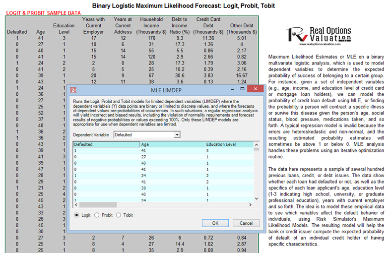
Figure 11.20: Maximum Likelihood Models