File Name: Decision Analysis – Expected Utility Analysis
Location: Modeling Toolkit | Decision Analysis | Expected Utility Analysis
Brief Description: Constructs a utility function using risk preferences and expected value of payoffs for a decision maker, as an alternative to expected value analysis
Requirements: Modeling Toolkit
This model applies utility theory in decision analysis to determine which projects should be executed given that the projects are risky and carry with them the potential for significant gains as well as significant losses. Using a single-point estimate or expected value given various probabilities of events occurring may not be the best approach. An alternative approach is to determine the risk preferences of the decision maker through the construction of a utility curve. Using the utility curve, we can then determine which project or strategy may best fit the decision-maker’s risk preferences.
The first portion of the model looks at the payoff table under three scenarios (high, moderate, and low prices) and their respective payoffs for three strategies (execute Project A, execute Project B, or do nothing). The expected value shows that Project A has the highest payoff. Hence, the best decision is to execute Project A.
However, if the company is a small start-up firm and the owner or decision maker is fairly risk averse (e.g., even a small loss of, say, $30,000 can potentially mean that the business faces bankruptcy). Under such circumstances, executing Project A may not be the best alternative. To analyze this situation, we revert to the use of utility functions. To start off, as an example, suppose we have a project where the maximum payoff on all strategies is $50,000 and the minimum is –$50,000. We construct a graduated set of payoffs from these two values and call them the guaranteed payoff (Figure 27.1). Then the decision maker is to determine the indifference probability (the maximum is always set to 100% whereas the minimum value is always set to 0%). Gradually moving down the payoffs, determine the indifference levels. For instance, say there is a coin toss game where if heads appear, you receive $50,000 versus a loss of –$50,000 if tails appear. This game yields an expected value of $0. In such a scenario, what is the probability you will accept $40,000 guaranteed versus playing the risky game? In the example, the decision maker sets the chances as 97%, and so forth. As another example, the decision maker is willing to accept a sure thing of $10,000 about 85% of the time rather than take the gamble of losing –$50,000 although the upside of $50,000 is still a potential.
From the risk-averse utility function generated, we can then recompute the payoff table by converting the monetary payoffs to utility payoffs. In this example, it is clear that both projects are fairly risky to the owner and the best course of action is to stay away from both projects. For more examples on decision analysis, see the Decision Analysis – Decision Tree with EVPI, Minimax and Bayes’ Theorem model. In addition, for more advanced decision analysis and strategies, see the real options analysis models and cases in Parts II and III of this book.
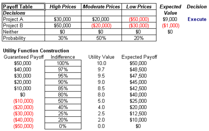
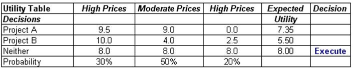
Figure 27.1: Expected utility analysis