The Kolmogorov–Smirnov (KS) test is a nonparametric test based on the empirical distribution function of a sample dataset. This nonparametric characteristic is the key to understanding the KS test, which simply means that the distribution of the KS test statistic does not depend on the underlying cumulative distribution function being tested. Nonparametric simply means no predefined distributional parameters are required. In other words, the KS test is applicable across a multitude of underlying distributions. Another advantage is that it is an exact test as compared to the chi-square test, which depends on an adequate sample size for the approximations to be valid. Despite these advantages, the KS test has several important limitations. It only applies to continuous distributions, and it tends to be more sensitive near the center of the distribution than at the distribution’s tails. Also, the distribution must be fully specified.
Given N ordered data points Y1, Y2, … YN, the empirical distribution function is defined as En = ni /N where ni is the number of points less than Yi where Yi are ordered from the smallest to the largest value. This is a step function that increases by 1/N at the value of each ordered data point. The null hypothesis is such that the dataset follows a specified distribution, while the alternate hypothesis is that the dataset does not follow the specified distribution. The hypothesis is tested using the KS statistic defined as![]() where F is the theoretical cumulative distribution of the continuous distribution being tested that must be fully specified (i.e., location, scale, and shape parameters cannot be estimated from the data).
where F is the theoretical cumulative distribution of the continuous distribution being tested that must be fully specified (i.e., location, scale, and shape parameters cannot be estimated from the data).
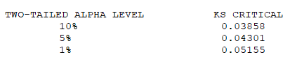
The hypothesis regarding the distributional form is rejected if the test statistic, KS, is greater than the critical value obtained from the table below. Notice that 0.03 to 0.05 are the most common levels of critical values (at the 1%, 5%, and 10% significance levels). Thus, any calculated KS statistic less than these critical values implies that the null hypothesis is not rejected and that the distribution is a good fit. There are several variations of these tables that use somewhat different scaling for the KS test statistic and critical regions. These alternative formulations should be equivalent, but it is necessary to ensure that the test statistic is calculated in a way that is consistent with how the critical values were tabulated. However, the rule of thumb is that a KS test statistic less than 0.03 or 0.05 indicates a good fit.