File Name: Volatility – Volatility Computations
Location: Modeling Toolkit | Volatility, and Applying Log Cash Flow Returns, Log Asset Returns, Probability to Volatility, EWMA, and GARCH Models
Brief Description: Uses Risk Simulator to apply Monte Carlo simulation to compute a project’s volatility measure
Requirements: Modeling Toolkit, Risk Simulator
There are several ways to estimate the volatility used in the option models. The most common and valid approaches are:
Logarithmic Cash Flow Returns Approach or Logarithmic Stock Price Returns Approach: This method is used mainly for computing the volatility of liquid and tradable assets, such as stocks in financial options. However, sometimes it is used for other traded assets, such as the price of oil or electricity. The drawback is that discounted cash flow models with only a few cash flows generally will overstate the volatility, and this method cannot be used when negative cash flows occur. Thus, this volatility approach is applicable only for financial instruments and not for real options analysis. The benefits include its computational ease, transparency, and modeling flexibility. In addition, no simulation is required to obtain a volatility estimate. The approach is simply to take the annualized standard deviation of the logarithmic relative returns of the time-series data as the proxy for volatility. The Modeling Toolkit function MTVolatility is used to compute this volatility, where the time series of stock prices can be arranged in either chronological or reverse chronological order when using the function. See the Log Cash Flow Returns example model in the Volatility section of Modeling Toolkit for details.
Exponentially Weighted Moving Average (EWMA) Models: This approach is similar to the logarithmic cash flow returns approach. It uses the MTVolatility function to compute the annualized standard deviation of the natural logarithms of relative stock returns. The difference here is that the most recent value will have a higher weight than values farther in the past. A lambda, or weight variable, is required (typically, industry standards set this at 0.94). The most recent volatility is weighted at this lambda value, and the period before that is (1 – lambda), and so forth. See the EWMA example model in the Volatility section of Modeling Toolkit for details.
Logarithmic Present Value Returns Approach: This approach is used mainly when computing the volatility on assets with cash flows. A typical application is in real options. The drawback of this method is that simulation is required to obtain a single volatility, and it is not applicable for highly traded liquid assets, such as stock prices. The benefits include the ability to accommodate certain negative cash flows. Also, this approach applies more rigorous analysis than the logarithmic cash flow returns approach, providing a more accurate and conservative estimate of volatility when assets are analyzed. In addition, within, say, a cash flow model, you can set up multiple simulation assumptions (insert any types of risks and uncertainties, such as related assumptions, correlated distributions and nonrelated inputs, multiple stochastic processes, etc.) and allow the model to distill all the interacting risks and uncertainties in these simulations. You then obtain the single-value volatility, which represents the integrated risk of the project. See the Log Asset Returns example model in the Volatility section of Modeling Toolkit for details.
Management Assumptions and Guesses: This approach is used for both financial options and real options. The drawback is that the volatility estimates are very unreliable and are only subjective best guesses. The benefit of this approach is its simplicity––using this method, you can easily explain to management the concept of volatility, both in execution and interpretation. Most people understand what probability is but have a hard time understanding what volatility is. Using this approach, you can impute one from another. See the Probability to Volatility example model in the Volatility section of Modeling Toolkit for details.
Generalized Autoregressive Conditional Heteroskedasticity (GARCH) Models: These methods are used mainly for computing the volatility of liquid and tradable assets, such as stocks in financial options. However, sometimes they are used for other traded assets, such as the price of oil or electricity. The drawback is that these models require a lot of data and advanced econometric modeling expertise is required. In addition, these models are highly susceptible to user manipulation. The benefit is that rigorous statistical analysis is performed to find the best-fitting volatility curve, providing different volatility estimates over time. The EWMA model is a simple weighting model; the GARCH model is a more advanced analytical and econometric model that requires advanced algorithms, such as the generalized method of moments, to obtain the volatility forecasts.
This chapter only provides a high-level review of all these methods as they pertain to hands-on applications. For detailed technical details on volatility estimates, including the theory and step-by-step interpretation of the method, please refer to Chapter 7 of Dr. Johnathan Mun’s Real Options Analysis, Third Edition (Thomson–Shore, 2016).
Procedure
-
- For the Log Cash Flow or Log Returns Approach, make sure that your data are all positive (this approach cannot apply negative values). The Log Cash Flow Approach worksheet illustrates an example computation of downloaded Microsoft stock prices (Figure 162.1). You can perform Edit | Copy and Edit | Paste Special | Values Only using your own stock closing prices to compute the volatility. The MTVolatility function is used to compute volatility. Enter in the positive integer for periodicity as appropriate (e.g., to annualize the volatility using monthly stock prices, enter in 12, or 52 for weekly stock prices, etc.), as seen in the example model.
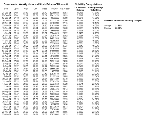
Figure 162.1 Historical stock prices and volatility estimates
- For the Log Present Value Approach, negative cash flows are allowed. In fact, this approach is preferred to the Log Cash Flow approach when modeling volatilities in a real options world. First, set some assumptions in the model or use the preset assumptions as is. The Intermediate X Variable is used to compute the project’s volatility (Figure 162.2). Run the simulation and view the Intermediate Variable X’s forecast chart. Go to the Statistics tab and obtain the Standard Deviation (Figure 162.3). Annualize it by multiplying the value with the square root of the number of periods per year (in this case, the annualized volatility is 11.64% as the periodicity is annual, otherwise multiply the standard deviation by the square root of 4 if quarterly data is used, the square root of 12 if monthly data is used, etc.).
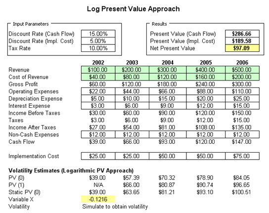
Figure 162.2: Using the PV Asset approach to model volatility
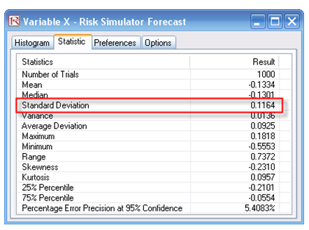
Figure 162.3: Volatility estimates using the PV Asset approach and simulation
- The Volatility to Probability approach can provide rough estimates of volatility, or you can use it to explain to senior management the concept of volatility. To illustrate, say your model has an expected value of $100M, and the best-case scenario as modeled or expected or anticipated by subject matter experts or senior management is $150M with a 10% chance of exceeding this value. We compute the implied volatility as 39.02% (Figure 162.4).
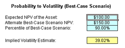
Figure 162.4: Probability to volatility approximation approach
Clearly, this is a rough estimate, but it is a good start if you do not wish to perform elaborate modeling and simulation to obtain a volatility measure. Further, this approach can be reversed. That is, instead of getting volatility from probability, you can get probability from volatility. This reversed method is very powerful in explaining to senior management the concept of volatility. To illustrate, we use the Worst-Case Scenario model next.
Suppose you run a simulation model and obtain an annualized volatility of 35% and need to explain what this means to management. Well, 35% volatility does not mean that there is a 35% chance of something happening, nor does it mean that the expected value can go up 35%, and so forth. Management has a hard time understanding volatility, whereas probability is a simpler concept. For instance, if you state that there is a 10% chance of something happening (such as a product being successful in the market), management understands this to mean that 1 out of 10 products will be a superstar. You can take advantage of this fact and impute the probability from the analytically computed volatility to explain the concept in a simplified manner. Using the Probability to Volatility Worst-Case Scenario model, assume that the worst-case is defined as the 10% left tail (you can change this if you wish), and that your analytical model provides a 35% volatility. Simply click on Tools | Goal Seek and set the cell F24 (the volatility cell) to change to the value 35% (your computed volatility) by changing the alternate worst-case scenario cell (F21). Clicking OK returns the value of $55.15 in cell F21. This means that a 35% volatility can be described as a project with an expected NPV of $100M. It is risky enough that the worst-case scenario can occur less than 10% of the time, and if it does, it will reduce the project’s NPV to $55.15M. In other words, there is a 1 in 10 chance the project will be below $55.15M, or 9 out of 10 times it will make at least $55.15M (Figure 162.5).
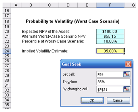
Figure 162.5: Sample computation using the volatility to probability approach
- For the EWMA and GARCH approaches, time-specific multiple volatility forecasts are obtained. That is, a term structure of volatility can be determined using these approaches. GARCH models are used mainly in analyzing financial time-series data, in order to ascertain their conditional variances and volatilities. These volatilities are then used to value the options as usual, but the amount of historical data necessary for a good volatility estimate remains significant. Usually, several dozen—and even up to hundreds—of data points are required to obtain good GARCH estimates. GARCH is a term that incorporates a family of models that can take on a variety of forms, known as GARCH(p,q), where p and q are positive integers that define the resulting GARCH model and its forecasts. In most cases for financial instruments, a GARCH(1,1) is sufficient and is most generally used.For instance, a GARCH (1,1) model takes the form of
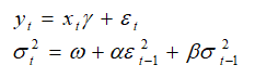
where the first equation’s dependent variable (yt) is a function of exogenous variables (xt) with an error term (εt). The second equation estimates the variance (squared volatility σt2) at time t, which depends on a historical mean (ω), news about volatility from the previous period, measured as a lag of the squared residuals from the mean equation (εt-12), and volatility from the previous period (σt-12). The exact modeling specification of a GARCH model is beyond the scope of this book. Suffice it to say that detailed knowledge of econometric modeling (model specification tests, structural breaks, and error estimation) is required to run a GARCH model, making it less accessible to the general analyst. The other problem with GARCH models is that the model usually does not provide a good statistical fit. That is, it is impossible to predict the stock market and, of course, equally if not harder to predict a stock’s volatility over time. Figure 162.6 shows a GARCH (1,1) on a sample set of historical stock prices using the MTGARCH model.
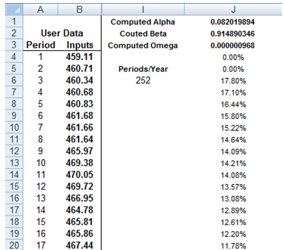
Figure 162.6: Sample GARCH (1,1) model
In order to create GARCH forecasts, start the Modeling Toolkit and open the Volatility | GARCH model. You will see a model that resembles Figure 162.7. Follow the next procedures to create the volatility estimates:
- Enter the Stock Prices in chronological order (e.g., cells I6:I17).
- Use the MTGARCH function call in Modeling Toolkit. For instance, cell K3 has the function call “MTGARCH($I$6:$I$17,$I$19,1,3)” where the stock price inputs are in cells I6:I17, the periodicity is 12 (i.e., there are 12 months in a year, to obtain the annualized volatility forecasts), and the predictive base is 1, and we forecast for a sample of 3 periods into the future. Because we will copy and paste the function down the column, make sure that absolute addressing is used, i.e., $I$6 and not relative addressing I6.
- Copy cell K3 and paste the function on cells K3:K20 (select cell K3 and drag the fill handle to copy the function down the column). You do this because the first three values are the GARCH estimated parameters of Alpha, Beta, and Gamma, and at the bottom (e.g., cells K18:K20) are the forecast values.
- With the entire column selected (cells K3:K20 selected), hit F2 on the keyboard, and then hold down Shift + Ctrl and hit Enter. This will update the entire matrix with GARCH forecasts.
Alternatively, and probably a simpler method, is to use Risk Simulator’s Forecast GARCH module as seen in Figure 162.8, select the data location of raw stock prices, and enter in the required parameters (see below for a description of these parameters). The result is a GARCH volatility report seen in Figure 162.9.
Note that the GARCH function has several inputs as follow:
Stock Prices: This is the time series of stock prices in chronological order. Typically, dozens of data points are required for a decent volatility forecast.
Periodicity: This is a positive integer indicating the number of periods per year (e.g., 12 for monthly data, 252 for daily trading data, etc.), assuming you wish to annualize the volatility. For getting periodic volatility, enter 1.
Predictive Base: This is the number of periods (the time-series data) back to use as a base to forecast volatility. The higher this number, the longer the historical base is used to forecast future volatility.
Forecast Period: This is a positive integer indicating how many future periods beyond the historical stock prices you wish to forecast.
Variance Targeting: This variable is set as False by default (even if you do not enter anything here) but can be set as True. False means the omega variable is automatically optimized and computed. The suggestion is to leave this variable empty. If you wish to create mean-reverting volatility with variance targeting, set this variable as True.
P: This is the number of previous lags on the mean equation.
Q: This is the number of previous lags on the variance equation.
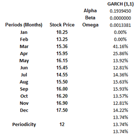
Figure 162.7: Setting up a GARCH model
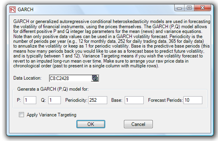
Figure 162.8: Running a GARCH model in Risk Simulator
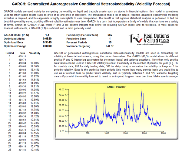
Figure 162.9: GARCH forecast results
- For the Log Cash Flow or Log Returns Approach, make sure that your data are all positive (this approach cannot apply negative values). The Log Cash Flow Approach worksheet illustrates an example computation of downloaded Microsoft stock prices (Figure 162.1). You can perform Edit | Copy and Edit | Paste Special | Values Only using your own stock closing prices to compute the volatility. The MTVolatility function is used to compute volatility. Enter in the positive integer for periodicity as appropriate (e.g., to annualize the volatility using monthly stock prices, enter in 12, or 52 for weekly stock prices, etc.), as seen in the example model.