File Name: Optimization – Capital Investments (Part A)
Location: Modeling Toolkit | Optimization | Investment Capital Allocation – Part I
Brief Description: Finds the optimal levels of capital investments in a strategic plan based on different risk and return characteristics of each type of product lines (the first of a two-part model)
Requirements: Modeling Toolkit, Risk Simulator
Companies restructure their product mix to boost sales and profits, increase shareholder value, or survive when the corporate structure becomes impaired. In successful restructurings, management not only actualizes lucrative new projects, but also abandons existing projects when they no longer yield sufficient returns, thereby channeling resources to more value-creating uses. At one level, restructuring can be viewed as changes in financing structures and management. At another level, it may be operational—in response to production overhauls, market trends, technology, and the industry or macroeconomic disturbances.
For banks called on to finance corporate restructurings, things are a bit different. For example, most loans provide a fixed return over fixed periods that are dependent on interest rates and the borrower’s ability to pay. A good loan will be repaid on time and in full. Hopefully, the bank’s cost of funds will be low, with the deal providing attractive risk-adjusted returns. If the borrower’s business excels, the bank will not participate in upside corporate values (except for a vicarious pleasure in the firm’s success). However, if a borrower ends up financially distressed, lenders share much and perhaps most of the pain.
Two disparate goals—controlling default (credit) risk, the bank’s objective, and value maximization, a traditional corporate aspiration—are often at odds, particularly if borrowers want the money to finance excessively aggressive projects. In the vast majority of traditional credit analyses, where the spotlight focuses on deterministically drawn projections, hidden risks are often exceedingly difficult to uncover. Devoid of viable projections, bankers will time and again fail to bridge gaps between their agendas and client aspirations. This chapter and the next offer ways for bankers to advance both their analytics and their communication skills; senior bank officials and clients alike, to “get the deal done” and ensure risk/reward agendas, are set in equilibrium. Undeniably, the direct way to achieve results is to take a stochastic view of strategic plans rather than rely inappropriately on a deterministic base case/conservative scenarios.
ABC Bank is asked to approve a $3,410,000 loan facility for the hypothetical firm RI Furniture Manufacturing LTD. Management wants to restructure four of its operating subsidiaries. In support of the facility, the firm supplied the bank with deterministic base-case and conservative consolidating and consolidated projections—income statement, balance sheet, and cash flows. On the basis of deterministic consolidating projections, bankers developed the stochastic spreadsheet depicted in Figure 98.1. This spreadsheet includes maximum/minimum investments ranges supporting restructuring in each of the four product lines, and Risk Simulator is applied to run an optimization on the optimal amounts to invest in each product line. The annual operating returns are also set as assumptions in a stochastic optimization run. To run the Optimization in the preset model, click on Risk Simulator | Optimization | Run Optimization or click on the Run Optimization icon and select Stochastic Optimization. Figure 98.2 illustrates the results without (before) and with (after) optimization. Notice that the expected returns have increased through an optimal allocation of the investments in the four business units.
Figure 98.3 shows the results of two simulation runs (simulation is run on the original before-optimization allocation and is then rerun after the optimization). As expected, the mean or expected returns is higher with the optimization, but because we only set the total returns as the objective, risks also went up (as measured by standard deviation) by virtue of higher returns necessitating higher risks. However, at closer inspection, the coefficient of variation, which is computed by the standard deviation divided by the mean (risk to return ratio), actually stayed relatively constant (the small variations are due to random effects of simulation, which will dissipate with higher simulation trials).
Typically, at this point, as a prudent next step, the banker will have to discuss this first optimization run with the firm’s management on three levels: the maximum expected return, the optimal investments/loan facility allocation, and the risk of expected returns. If the risk level is unacceptable, the standard deviation must be reduced to preserve credit grade integrity. In the next chapter, we take this simple model and add more levels of complexity by adding in an efficient frontier model and credit risk contribution effects on the portfolio.
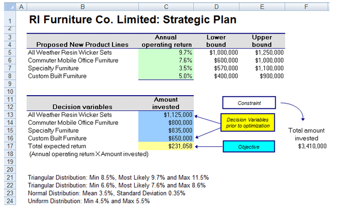
Figure 98.1: Investment allocation model
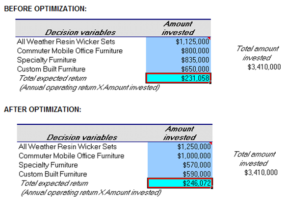
Figure 98.2: Results from before and after an optimization run
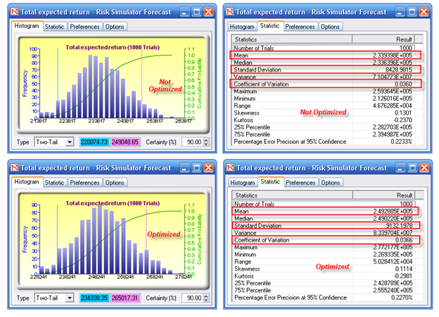
Figure 98.3: Simulation results from before and after an optimization