File Name: Forecasting – Time-Series ARIMA
Location: Modeling Toolkit | Forecasting | Time-Series ARIMA
Brief Description: Illustrates how to run an econometric model called the Box-Jenkins ARIMA, which stands for autoregressive integrated moving average, an advanced forecasting technique that takes into account historical fluctuations, trends, seasonality, cycles, prediction errors, and nonstationarity of the data
Requirements: Modeling Toolkit, Risk Simulator
The Data worksheet in the model contains some historical time-series data on money supply in the United States, denoted M1, M2, and M3. M1 is the most liquid form of money (cash, coins, savings accounts, etc.); M2 and M3 are less liquid forms of money (bearer bonds, certificates of deposit, etc.). These datasets are useful examples of long-term historical time-series data where ARIMA can be applied.
Briefly, ARIMA econometric modeling takes into account historical data and decomposes it into an Autoregressive (AR) process, where there is a memory of past events (e.g., the interest rate this month is related to the interest rate last month, and so forth, with a decreasing memory lag); an Integrated (I) process, which accounts for stabilizing or making the data stationary and ergodic, making it easier to forecast; and a Moving Average (MA) of the forecast errors, such that the longer the historical data series, the more accurate the forecasts will be, as the model learns over time. ARIMA models, therefore, have three model parameters: one for the AR(p) process, one for the I(d) process, and one for the MA(q) process, all combined and interacting among each other and recomposed into the ARIMA (p,d,q) model.
There are many reasons why an ARIMA model is superior to ordinary time-series analysis and multivariate regressions. The common finding in time-series analysis and multivariate regression is that the error residuals are correlated with their own lagged values. This serial correlation violates the standard assumption of regression theory that disturbances are not correlated with other disturbances. The primary problems associated with serial correlation are:
- Regression analysis and basic time-series analysis are no longer efficient among the different linear estimators. However, as the error residuals can help to predict current error residuals, we can take advantage of this information to form a better prediction of the dependent variable using ARIMA.
- Standard errors computed using the regression and time-series formula are not correct and are generally understated. If there are lagged dependent variables set as the regressors, regression estimates are biased and inconsistent but can be fixed using ARIMA.
Autoregressive Integrated Moving Average or ARIMA(p,d,q) models are the extensions of the AR model that uses three components for modeling the serial correlation in the time-series data. The first component is the autoregressive (AR) term. The AR(p) model uses the p lags of the time series in the equation. An AR(p) model has the form: yt = a1yt-1 + … + apyt-p + et. The second component is the integration (d) order term. Each integration order corresponds to differencing the time series. I(1) means differencing the data once. I(d) means differencing the data d times. The third component is the moving average (MA) term. The MA(q) model uses the q lags of the forecast errors to improve the forecast. An MA(q) model has the form: yt = et + b1et-1 + … + bqet-q. Finally, an ARMA(p,q) model has the combined form: yt = a1 yt-1 + … + a p yt-p + et + b1 et-1 + … + bq et-q.
In interpreting the results of an ARIMA model, most of the specifications are identical to the multivariate regression analysis. However, there are several additional sets of results specific to the ARIMA analysis. The first is the addition of Akaike Information Criterion (AIC) and Schwarz Criterion (SC), which are often used in ARIMA model selection and identification. That is, AIC and SC are used to determine if a particular model with a specific set of p, d, and q parameters is a good statistical fit. SC imposes a greater penalty for additional coefficients than the AIC, but generally, the model with the lowest AIC and SC values should be chosen. Finally, an additional set of results called autocorrelation (AC), and partial autocorrelation (PAC) statistics is provided in the ARIMA report.
For instance, if autocorrelation AC(1) is nonzero, it means that the series is first-order serially correlated. If AC dies off more or less geometrically with increasing lags, it implies that the series follows a low-order autoregressive process. If AC drops to zero after a small number of lags, it implies that the series follows a low-order moving-average process. In contrast, PAC measures the correlation of values that are k periods apart after removing the correlation from the intervening lags. If the pattern of autocorrelation can be captured by an autoregression of order less than k, then the partial autocorrelation at lag k will be close to zero. The Ljung-Box Q-statistics and their p-values at lag k are also provided, where the null hypothesis being tested is such that there is no autocorrelation up to order k. The dotted lines in the plots of the autocorrelations are the approximate two standard error bounds. If the autocorrelation is within these bounds, it is not significantly different from zero at approximately the 5% significance level.
Finding the right ARIMA model takes practice and experience. These AC, PAC, SC, and AIC are highly useful diagnostic tools to help identify the correct model specification. Finally, the ARIMA parameter results are obtained using sophisticated optimization and iterative algorithms, which means that although the functional forms look like those of multivariate regression, they are not the same. ARIMA is a much more computationally intensive and advanced econometric approach.
Running a Monte Carlo Simulation
To run this model, simply:
- Go to the Data worksheet and select Risk Simulator | Forecasting | ARIMA.
- Click on the link icon beside the Time Series Variable input box, and link in C7:C442.
- Enter in the relevant P, D, Q inputs, forecast periods, maximum iterations, and so forth (Figure 90.1) and click OK.
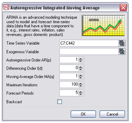
Figure 90.1: Running a Box-Jenkins ARIMA model
The nice thing about using Risk Simulator is the ability to run its Auto-ARIMA module. That is, instead of needing advanced econometric knowledge, the Auto-ARIMA module can automatically test all most commonly used models and rank them from the best fit to the worst fit. Figure 90.2 illustrates the results generated from an Auto-ARIMA module in Risk Simulator and Figure 90.3 shows the best-fitting ARIMA model report. Finally, please note that if the Exogenous Variable input is used, the number of data points in this variable less the number of data points in the Time-Series Variable has to exceed the number of Forecast Periods.
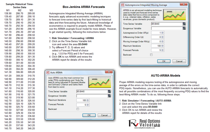
Figure 90.2: Auto-ARIMA model
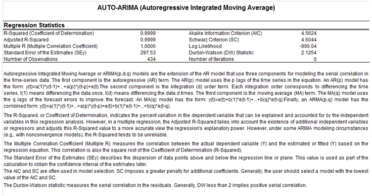
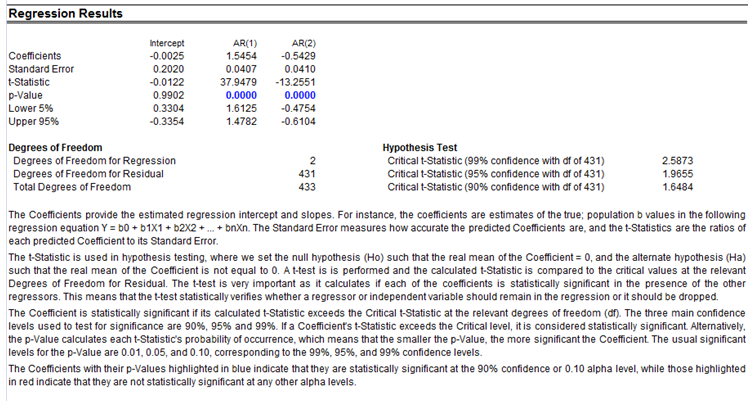
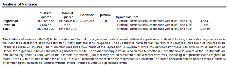
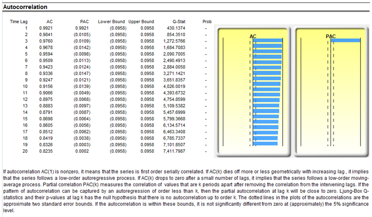
Figure 90.3: Auto-ARIMA results