Additive Seasonality
If the time-series data have no appreciable trend but exhibit seasonality, then the additive seasonality and multiplicative seasonality methods apply. The additive seasonality method is illustrated in Figures 12.14 and 12.15.
The additive seasonality model breaks the historical data into a level (L) or base-case component as measured by the alpha parameter (α), and a seasonality (S) component measured by the gamma parameter (γ). The resulting forecast value is simply the addition of this base case level to the seasonality value. (Please be aware that all calculations are rounded). Quarterly seasonality is assumed in the example.
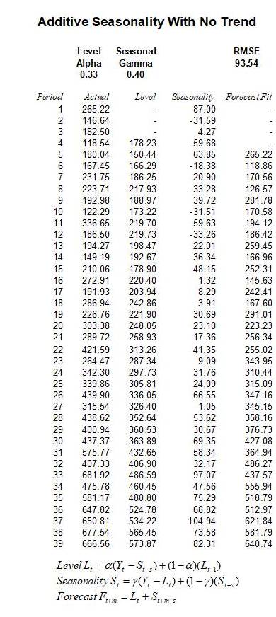
Figure 12.14: Seasonal Additive (Seasonality = 4)
As explained, when there is seasonality in the data but a trend does not exist, the seasonal additive (Figure 12.14) or seasonal multiplicative (Figure 12.15) models may be appropriate. The main difference between these two approaches is that the additive model uses addition and subtraction versus multiplication and division, and, of course, the optimized α and γ parameters would also be different to compensate for these differences in mathematical operations.
Figure 12.14 shows the model setup for a seasonal additive model and Figure 12.15 explores in more detail the actual computations. Typically, to get started, the Actual column lists the historical time-series data in chronological order. The data in this example has a seasonality of 4 periods (i.e., quarterly data where there are 4 quarters in a year, representing one full cycle) the Level column starts on period 4 (the seasonality) and the forecast fit which is one period forecast out, starts at period 5.
For the Level calculations, the first value is simply the average of the previous Actual values for the entire season. As the seasonality in this example is 4, the first Level value is computed as the average of 265.22, 146.64, 182.5, and 118.54 or 178.23. Starting from![]() onwards, the Level is computed using the equation in Figure 12.14, where we compute
onwards, the Level is computed using the equation in Figure 12.14, where we compute![]()
(rounded). Note that in this case the optimized α is 0.3261, the ![]() represents the actual historical data point for the same period t,
represents the actual historical data point for the same period t, ![]() represents the Seasonality value s periods back from period t (s = 4 in this example), and
represents the Seasonality value s periods back from period t (s = 4 in this example), and![]() represents the previous period’s calculated Level (i.e., 178.23 in this example). All subsequent values in the Level column are calculated the same way.
represents the previous period’s calculated Level (i.e., 178.23 in this example). All subsequent values in the Level column are calculated the same way.
For the Seasonality calculations, as there are 4 periods in this season, the first 4 figures are computed using the![]() for the first seasonality value, 146.64 – 178.23 = –31.59 for the second period, and so forth, until the fourth period (or whatever period, depending on the seasonality of the data). All Seasonality calculations after the first s periods are computed using the equation seen in Figure 12.15. For instance, period 5’s Seasonality factor is computed as
for the first seasonality value, 146.64 – 178.23 = –31.59 for the second period, and so forth, until the fourth period (or whatever period, depending on the seasonality of the data). All Seasonality calculations after the first s periods are computed using the equation seen in Figure 12.15. For instance, period 5’s Seasonality factor is computed as![]() Finally, the Forecast Fit model is calculated one period out at a time. As an example, the period 5 Forecast Fit value is computed as
Finally, the Forecast Fit model is calculated one period out at a time. As an example, the period 5 Forecast Fit value is computed as ![]() All subsequent periods are calculated in the same fashion going forward. For future forecast periods beyond the seasonality periodicity (i.e., seasonality in this example is 4, which means we can use the last 4 periods’ seasonality factors in forecasting periods 40 – 43, but for periods 44 onward, we call this beyond the historical seasonality period), we replicate the last seasonality factors. This means that the confidence in future forecasts beyond the seasonality periodicity will be less accurate in general, due to insufficient seasonal data, and we, therefore, assume that the seasonality will repeat itself going forward. This is clearly one of the shortcomings of the current methodology.
All subsequent periods are calculated in the same fashion going forward. For future forecast periods beyond the seasonality periodicity (i.e., seasonality in this example is 4, which means we can use the last 4 periods’ seasonality factors in forecasting periods 40 – 43, but for periods 44 onward, we call this beyond the historical seasonality period), we replicate the last seasonality factors. This means that the confidence in future forecasts beyond the seasonality periodicity will be less accurate in general, due to insufficient seasonal data, and we, therefore, assume that the seasonality will repeat itself going forward. This is clearly one of the shortcomings of the current methodology.
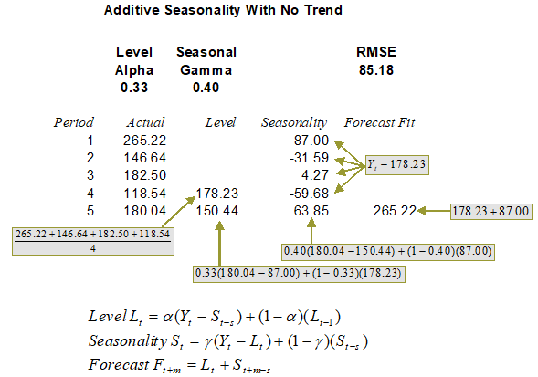
Figure 12.15: Calculating Seasonal Additive
Multiplicative Seasonality
Similarly, the multiplicative seasonality model requires the alpha and gamma parameters. The difference is that the model is multiplicative, for example, the forecast value is the multiplication between the base case level and seasonality factor. Figures 12.16 and 12.17 illustrate the computations required. Quarterly seasonality is assumed in the example. (Please be aware that all calculations are rounded).
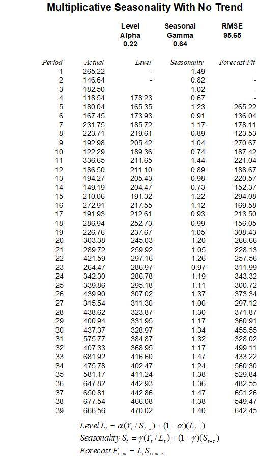
Figure 12.16: Seasonal Multiplicative
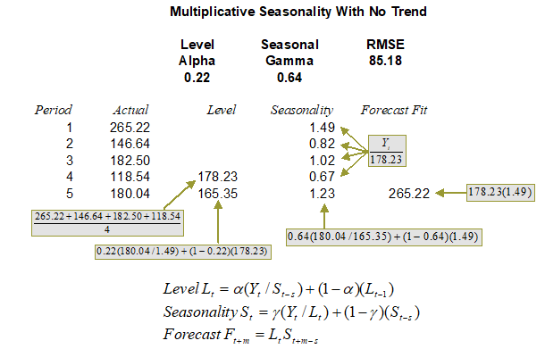
Figure 12.17: Calculating Seasonal Multiplicative (Seasonality = 4)