File Name: Risk Analysis – Integrated Risk Analysis
Location: Modeling Toolkit | Risk Analysis | Integrated Risk Analysis
Brief Description: Integrates Monte Carlo simulation, forecasting, portfolio optimization, and real options analysis into a single unified model and shows how one plays off the other
Requirements: Modeling Toolkit, Risk Simulator
Before diving into the different risk analysis methods in the remaining chapters of the book, it is important to first understand Integrated Risk Management (IRM) and how these different techniques are related in a risk analysis and risk management context. This IRM framework comprises eight distinct phases of a successful and comprehensive risk analysis implementation, going from a qualitative management screening process to creating clear and concise reports for management. The process was developed by the author based on previous successful implementations of risk analysis, forecasting, real options, valuation, and optimization projects both in the consulting arena and in industry-specific problems. These phases can be performed either in isolation or together in a sequence for a more robust integrated analysis. Figure 121.1 shows the Integrated Risk Management process up close. We can separate the process into the following eight simple steps:
- Qualitative Management Screening
- Forecast Predictive Modeling
- Base Case Static Model
- Monte Carlo Risk Simulation
- Real Options Problem Framing
- Real Options Valuation and Modeling
- Portfolio and Resource Optimization
- Reporting, Presentation, and Update Analysis
1. Qualitative Management Screening
Qualitative management screening is the first step in any Integrated Risk Management process. Management has to decide which projects, assets, initiatives, or strategies are viable for further analysis, in accordance with the firm’s mission, vision, goal, or overall business strategy. The firm’s mission, vision, goal, or overall business strategy may include market penetration strategies, and competitive advantage, technical, acquisition, growth, synergistic, or globalization issues. That is, the initial list of projects should be qualified in terms of meeting management’s agenda. Often the most valuable insight is created as management frames the complete problem to be resolved. This is where the various risks to the firm are identified and fleshed out.
2. Forecast Predictive Modeling
The future is then forecasted using time-series analysis or multivariate regression analysis if historical or comparable data exist. Otherwise, other qualitative forecasting methods may be used (subjective guesses, growth rate assumptions, expert opinions, Delphi method, etc.). In a financial context, this is the step where future revenues, sale price, quantity sold, volume, production, and other key revenue and cost drivers are forecasted. See Chapter 9 of Modeling Risk, Third Edition, for details on forecasting and using the author’s Risk Simulator software to run time-series, nonlinear extrapolation, stochastic process, ARIMA, multivariate regression forecasts, fuzzy logic, neural networks, econometric models, GARCH, and so on.
3. Base Case Static Model
For each project that passes the initial qualitative screens, a discounted cash flow model is created. This model serves as the base case analysis where a net present value is calculated for each project, using the forecasted values in the previous step. This step also applies if only a single project is under evaluation. This net present value is calculated using the traditional approach of modeling and forecasting revenues and costs, and discounting the net of these revenues and costs at an appropriate risk-adjusted rate. The return on investment and other profitability, cost-benefit, and productivity metrics are generated here.
4. Monte Carlo Risk Simulation
Because the static discounted cash flow produces only a single-point estimate result, there is oftentimes little confidence in its accuracy given that future events that affect forecast cash flows are highly uncertain. To better estimate the actual value of a particular project, Monte Carlo risk simulation should be employed next
Usually, a sensitivity analysis is first performed on the discounted cash flow model; that is, setting the net present value as the resulting variable, we can change each of its precedent variables and note the change in the resulting variable. Precedent variables include revenues, costs, tax rates, discount rates, capital expenditures, depreciation, and so forth, which ultimately flow through the model to affect the net present value figure. By tracing back all these precedent variables, we can change each one by a preset amount and see the effect on the resulting net present value. A graphical representation can then be created, which is oftentimes called a tornado chart because of its shape, where the most sensitive precedent variables are listed first, in descending order of magnitude. Armed with this information, the analyst can then decide which key variables are highly uncertain in the future and which are deterministic. The uncertain key variables that drive the net present value and, hence, the decision are called critical success drivers. These critical success drivers are prime candidates for Monte Carlo simulation. Because some of these critical success drivers may be correlated––for example, operating costs may increase in proportion to quantity sold of a particular product, or prices may be inversely correlated to quantity sold––a correlated Monte Carlo simulation may be required. Typically, these correlations can be obtained through historical data. Running correlated simulations provides a much closer approximation to the variables’ real-life behaviors.
5. Real Options Problem Framing
After quantifying risks in the previous step, the question now is, what’s next? The risk information obtained somehow needs to be converted into actionable intelligence. So what if risk has been quantified to be such and such using Monte Carlo simulation? What do we do about it? The answer is to use real options analysis to hedge these risks, to value these risks, and to position yourself to take advantage of the risks. The first step in real options is to generate a strategic map through the process of framing the problem. Based on the overall problem identification occurring during the initial qualitative management screening process, certain strategic optionalities would have become apparent for each particular project. The strategic optionalities may include, among other things, the option to expand, contract, abandon, switch, choose, and so forth. Based on the identification of strategic optionalities that exist for each project or at each stage of the project, the analyst can then choose from a list of options to analyze in more detail. Real options are added to the projects to hedge downside risks and to take advantage of upside swings.
6. Real Options Valuation and Modeling
Through the use of Monte Carlo risk simulation, the resulting stochastic discounted cash flow model will have a distribution of values. Thus, simulation models, analyzes, and quantifies the various risks and uncertainties of each project. The result is a distribution of the NPVs and the project’s volatility. In real options, we assume that the underlying variable is the future profitability of the project, which is the future cash flow series. An implied volatility of the future free cash flow or underlying variable can be calculated through the results of a Monte Carlo simulation previously performed. Usually, the volatility is measured as the standard deviation of the logarithmic returns on the free cash flow stream (other approaches include running GARCH models and using simulated coefficients of variation as proxies). In addition, the present value of future cash flows for the base case discounted cash flow model is used as the initial underlying asset value in real options modeling. Using these inputs, real options analysis is performed to obtain the projects’ strategic option values.
7. Portfolio and Resource Optimization
Portfolio optimization is an optional step in the analysis. If the analysis is done on multiple projects, management should view the results as a portfolio of rolled-up projects because the projects are, in most, cases correlated with one another, and viewing them individually will not present the true picture. As firms do not only have single projects, portfolio optimization is crucial. Given that certain projects are related to others, there are opportunities for hedging and diversifying risks through a portfolio. Because firms have limited budgets, as well as time and resource constraints, while at the same time have requirements for certain overall levels of returns, risk tolerances, and so forth, portfolio optimization takes into account all these to create an optimal portfolio mix. The analysis will provide the optimal allocation of investments across multiple projects.
8. Reporting, Presentation, and Update Analysis
The analysis is not complete until reports can be generated. Not only are results presented, but the process should also be shown. Clear, concise, and precise explanations transform a difficult black-box set of analytics into transparent steps. Management will never accept results coming from black boxes if it does not understand where the assumptions or data originate and what types of mathematical or financial massaging take place.
Risk analysis assumes that the future is uncertain and that management has the right to make midcourse corrections when these uncertainties become resolved or risks become known; the analysis is usually done ahead of time and thus, ahead of such uncertainty and risks. Therefore, when these risks become known, the analysis should be revisited to incorporate the decisions made or to revise any input assumptions. Sometimes, for long-horizon projects, several iterations of the real options analysis should be performed, where future iterations are updated with the latest data and assumptions. Understanding the steps required to undertake an Integrated Risk Management analysis is important because it provides insight not only into the methodology itself but also into how it evolves from traditional analyses, showing where the traditional approach ends and where the advanced analytics start.
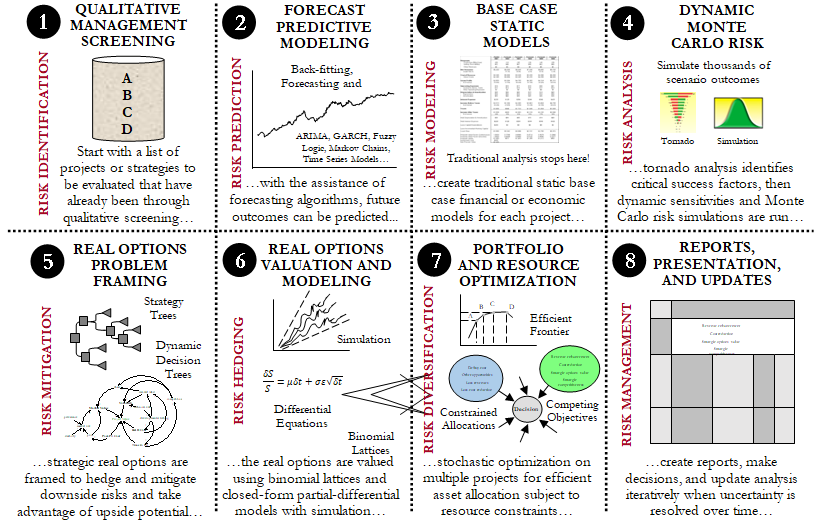
Figure 121.1: Visual representation of the Integrated Risk Management Process
Forecasting
In the Forecasting worksheet (Figure 121.2), first, create a profile (Risk Simulator | New Profile) and give it a name, then select the area G7:G26 of the data area and click on Risk Simulator | Forecasting | Time-Series Analysis. Suppose you know from experience that the seasonality of the revenue stream peaks every four years. Enter the seasonality of 4 and specify the number of forecast periods to 5. The Forecasting tool automatically selects the best time-series model to forecast the results through backcast-fitting techniques and optimization, to find the best-fitting model and its associated parameters. The best-fitting time-series analysis model is chosen. Running this module on the historical data will generate a report with the five-year forecast revenues (Forecast Report worksheet) that are complete with Risk Simulator assumptions (cells D43:D47). These output forecasts then become the inputs into the Valuation Model worksheet (cells D19:H19).
Monte Carlo Simulation
The Valuation Model worksheet shows a simple discounted cash flow model (DCF) that calculates the relevant net present value (NPV) and internal rate of return (IRR) of a project or strategy. Notice that the output of the Forecast Report worksheet becomes an input into this Valuation Model worksheet. For instance, cells D19:H19 are linked from the first forecast worksheet. The model uses two discount rates for the two different sources of risk (market risk-adjusted discount rate of 12% for the risky cash flows, and a 5% cost of capital to account for the private risk of capital investment costs). Further, different discounting conventions are included (midyear, end-year, continuous, and discrete discounting), as well as a terminal value calculation assuming a constant growth model. Finally, the capital implementation costs are separated out of the model (row 46), but the regular costs of doing business (direct costs, cost of goods sold, operating expenses, etc.) are included in the computation of free cash flows. That is, this project has two phases. The first phase costs $5 and the second larger phase costs $2,000.
The statistic NPV shows a positive value of $123.26 while the IRR is 15.68%, both exceeding the zero-NPV and firm-specific hurdle rate of 12% required rate of return. Therefore, at first pass, the project seems to be profitable and justifiable. However, risk has not been considered. Without applying risk analysis, you cannot determine the chances this NPV and IRR are expected to occur. This is done by selecting the cells you wish to simulate (e.g., D20) and clicking on Risk Simulator | Set Input Assumption (Figure 121.3). For illustration purposes, select the triangular distribution and link to the input parameters to the appropriate cells. Continue the process to define input assumptions on all other relevant cells. Then select the output cells such as NPV, IRR, and so forth (cells D14, D15, H14, and H15) and set them as forecasts (i.e., select each cell one at a time and click on Risk Simulator | Set Output Forecast and enter the relevant variable names). Note that all assumptions and forecasts have already been set for you.
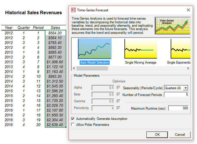
Figure 121.2: Stochastic time-series forecasting
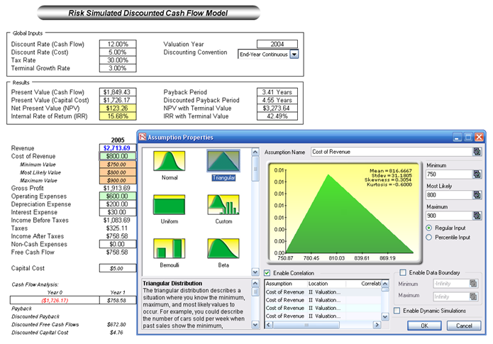
Figure 121.3: Applying Monte Carlo risk-based simulation on the model
Real Options Analysis
The next stop is real options analysis. In the previous simulation applications, risk was quantified and compared across multiple projects. The problem is, so what? That is, we have quantified the different levels of risks in different projects. Some are highly risky, some are somewhat risky, and some are not so risky. In addition, the relevant returns are also pretty variable as compared to the risk levels. Real options analysis takes this information to the next step. Looking at a specific project, real options identify if there are ways to mitigate the downside risks while taking advantage of the upside uncertainty. In applying Risk Simulator, we have only quantified uncertainties, not risks! Downside uncertainty, if it is real and affects the firm, becomes risks, while upside uncertainty is a plus that firms should try to capitalize on.
At this point, we can either solve real options problems using Real Options SLS’s multiple asset or MSLS module (install Real Options SLS and click on Start | Real Options Valuation | Real Options SLS | Real Options SLS) or apply its analytics directly in Excel by using the SLS Functions, which we will see later (Figures 121.5 and 121.6). The Real Options SLS is used to obtain a quick answer, but if a distribution of option values is required, then use the SLS Functions and link all the inputs into the function––we use the latter in this example. The real options analysis model’s inputs are the outputs from the DCF model in the previous step. For instance, the free cash flows are computed previously in the DCF. The Expanded NPV value in cell C21 in the Real Options worksheet is obtained through the SLS Function call. Simulation was used to also obtain the volatility required in the real options analysis.
The Real Options SLS results (Figure 121.4) indicate an Expanded NPV of $388M, while the NPV was $123M. This means that there is an additional $265 expected value in creating a two-staged development of this project rather than jumping in first and taking all the risk. That is, NPV analysis assumed that you would definitely invest all $5M in year 1 and $2,000M in year 3 regardless of the outcome (see Figure 121.7). This view of NPV analysis is myopic. Real options analysis, however, assumes that if all goes well in Phase I ($5M), then you continue on to Phase II ($2,000M). Therefore, due to the volatility and uncertainty in the project (as obtained by Monte Carlo simulation), there is a chance that the $2,000M may not even be spent, as Phase II never materializes (due to a bad outcome in Phase I). In addition, there is a chance that valuation free cash flows exceeding $1,849M may occur. The expected value of all these happenstances yields an Expanded NPV of $388M (the average potential after a two-phased stage-gate development process is implemented). It is better to perform a stage-gate development process than to take all the risks immediately and invest everything. Figures 121.5 and 126.6 illustrate how the analysis can be performed in the Excel model by using function calls.
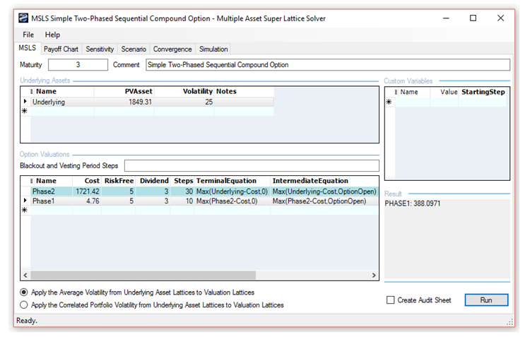
Figure 121.4: Applying real options on a two-phased project
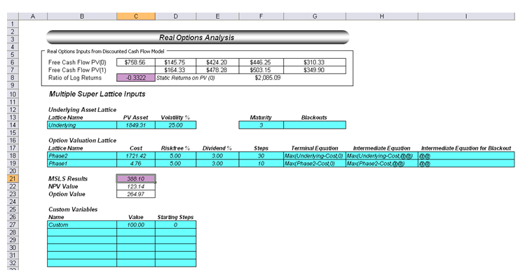
Figure 121.5: Linking real options in the spreadsheet
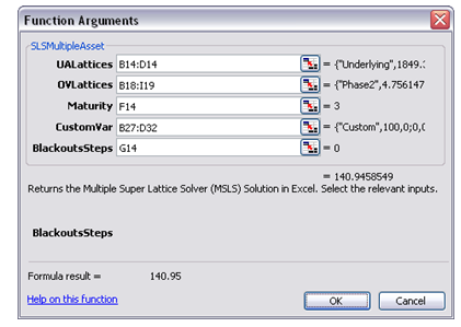
Figure 121.6: Real options function call in Excel
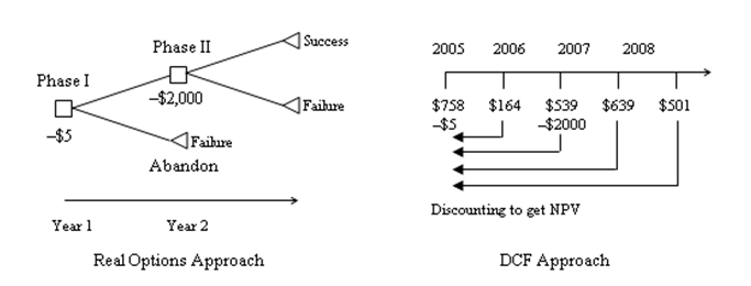
Figure 121.7: Graphical depiction of a two-phased sequential compound option model
Notice that in the real options world, executing Phase II is an option, not a requirement or obligation, while in the DCF world all investments have been decreed in advance and thus will and must occur (Figure 121.7). Therefore, management has the legitimate flexibility and ability to abandon the project after Phase I and not continue on to Phase II if the outcome of the first phase is bad. Based on the volatility calculated in the real options model, there is a chance Phase II will never be executed, there is a chance that the cash flows could be higher and lower, and there is a chance that Phase II will be executed if the cash flows make it profitable. Therefore, the net expected value of the project after considering all these potential avenues is the option value calculated previously. In this example as well, we assumed a 3% annualized dividend yield, indicating that by stage-gating the development and taking our time, the firm loses about 3% of its PV Asset per year (lost revenues and opportunity costs as well as lower market share due to waiting and deferring action).
Note that as dividends increase, the option to wait and defer action goes down. In fact, the option value reverts to the NPV value when dividends exceed 32%. That is, the NPV or value of executing now is $123.26M (i.e., $1849.43M – $1721.41M – $4.76M). So, at any dividend yield exceeding 32%, the optimal decision is to execute immediately rather than to wait and phase the development.
Optimization
The next step is portfolio optimization, that is, how to efficiently and effectively allocate a limited budget (budget constraint and human resource constraints) across many possible projects while simultaneously accounting for their uncertainties, risks, and strategic flexibility, and all the while maximizing the portfolio’s ENPV subject to the least amount of risk (Sharpe ratio). To this point, we have shown how a single integrated model can be built utilizing simulation, forecasting, and real options. Figure 121.8 illustrates a summary of 12 projects (here we assume that you have re-created the simulation, forecasting, and real options models for each of the other 11 projects), complete with their expanded NPV, NPV, cost, risk, return to risk ratio, and profitability index. To simplify our analysis and to illustrate the power of optimization under uncertainty, the returns and risk values for projects B to L are simulated, instead of rebuilding this 11 other times.
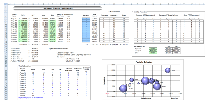
Figure 121.8: Portfolio of 12 projects with different risk-return profiles
Then the individual project’s human resource requirements as measured by full-time equivalences (FTEs) are included. We simplify the problem by listing only the three major human resource requirements: engineers, managers, and salespeople. The FTE salary costs are simulated using Risk Simulator. Finally, decision variables (the Decision Variables in column J in the model) are constructed, with a binary variable of 1 or 0 for a go and no-go decisions. The model also shows all 12 projects and their rankings sorted by returns, risk, cost, returns-to-risk ratio, and profitability ratio. Clearly, it is fairly difficult to determine simply by looking at this matrix which projects are the best to select in the portfolio.
The model also shows this matrix in graphical form, where the size of the balls is the cost of implementation, the x-axis shows the total returns including flexibility, and the y-axis lists the project risk as measured by volatility of the cash flows of each project. Again, it is fairly difficult to choose the right combinations of projects at this point. Optimization is required to assist in our decision making.
To set up the optimization process, first, select each of the decision variables in column J and set the relevant decision variables by clicking on Risk Simulator | Set Decision. Alternatively, you can create one decision variable and copy/paste. The linear constraint is such that the total budget value for the portfolio has to be less than $5,000. Next, select Portfolio Sharpe Ratio (D22) as the objective to maximize.
The next section illustrates the results of the optimization under uncertainty and the results interpretation. Further, we can add additional constraints if required such as where the total FTE cannot exceed $9,500,000, and so forth. We can then change the constraint of the number of projects allowed and we can marginally increase this constraint to see what additional returns and risks the portfolio will obtain. In each run, with a variable constraint inserted, an efficient frontier will be generated by connecting a sequence of optimal portfolios under different risk levels. That is, for a particular risk level, points on the frontier are the combinations of projects that maximize the returns of the portfolio subject to the lowest risk. Similarly, these are the points where, given a set of returns requirements, these combinations of projects provide the least amount of portfolio risk.
Optimization Parameters
For the first run, the following parameters were used:
Objective: Maximize Portfolio Returns
Constraint: Total Budget Allocation = $5,000
Constraint: Total number of projects not to exceed 6 (we then change this from 5 to 9, to create an investment efficient frontier)
The results, including a portfolio efficient frontier (Figure 121.9) where, on the frontier, all the portfolio combinations of projects will yield the maximum returns (portfolio NPV) subject to the minimum portfolio risks, are shown in Figure 121.10. Clearly, the first portfolio (with the 5-project constraint) is not a desirable outcome due to the low returns. So, the obvious candidates are the other portfolios. It is now up to management to determine what risk-return combination it wants; that is, depending on the risk appetite of the decision makers, the budget availability, and the capabilities of handling more projects, these five different portfolio combinations are the optimal portfolios of projects that maximize returns subject to the least risk, considering the uncertainties (simulation), strategic flexibility (real options), and uncertain future outcomes (forecasting). Of course, the results here are only for a specific set of input assumptions, constraints, and so forth. You may choose to change any of the input assumptions to obtain different variants of optimal portfolio allocations.
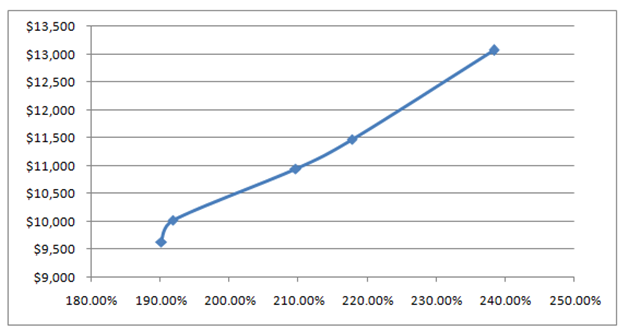
Figure 121.9: Efficient frontier
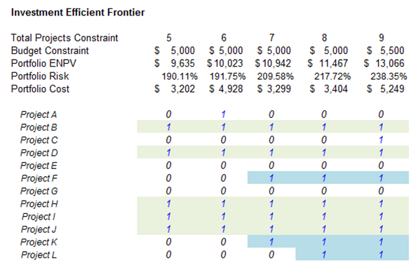
Figure 121.10: Project selection by multiple criteria
Many observations can be made from the summary of the results. While all of the optimal portfolios are constrained at under a total cost budget and the number of projects less than or equal to some value (in the efficient frontier, we change this constraint from 5 to 9 projects), all of these combinations of projects use the budget the most effectively as they generate the higher ENPV with the least amount of risk (Sharpe ratio is maximized) for the entire portfolio. However, the further on the right we go in the efficient frontier chart, the higher level of risk (wider range for ENPV and risk, higher volatility risk coefficient, requires more projects making it riskier, and higher total cost to implement) and the higher the returns. These values can be obtained from the forecast charts from Risk Simulator (not shown) by keeping the optimal project selections and running a simulation each time to view the ENPV and IRR forecast charts. It is at this point that the decision maker has to decide which risk-return profile to undertake.
All other combinations of projects in a portfolio are by definition suboptimal to these two, given the same constraints, and should not be entertained. Hence, from a possible portfolio combination of 12! or 479,000,000 possible outcomes, we have now isolated the decision down to these best portfolios. Finally, we can again employ a high-level portfolio real option on the decision. That is, because all portfolios require the implementation of projects B, D, H, I, J, do these first! Then leave the option open to execute the remaining projects (F, K, L) depending on which portfolios management decides to go with later. By doing so, we can buy additional time (portfolio level option to defer) before making the final determination, in case something happens during development, in which case the project can be terminated (option to abandon), the analysis can be rerun and different projects can be added, and new optimal portfolio can be obtained (option to switch).