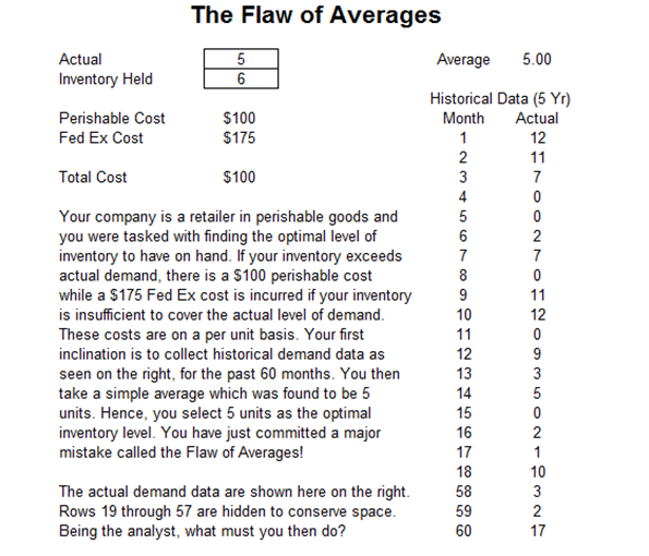
An example of why simulation is important can be seen in the case illustration in Figures 13.1 and 13.2, termed the Flaw of Averages. The example is most certainly worthy of more detailed study. It shows how an analyst may be misled into making the wrong decisions without the use of simulation. Suppose you are the owner of a shop that sells perishable goods and you need to make a decision on the optimal inventory to have on hand. Your new-hire analyst was successful in downloading 5-years’ worth of monthly historical sales levels and she estimates the average to be five units. You then make the decision that the optimal inventory to have on hand is five units. You have just committed the Flaw of Averages. As the example shows, the obvious reason why this error occurs is that the distribution of historical demand is highly skewed while the cost structure is asymmetrical. For example, suppose you are in a meeting, and your boss asks what everyone made last year. You take a quick poll and realize that the salaries range from $60,000 to $150,000. You perform a quick calculation and find the average to be $100,000. Then, your boss tells you that he made $20 million last year! Suddenly, the average for the group becomes $1.5 million. This value of $1.5 million clearly in no way represents how much each of your peers made last year. In this case, the median may be more appropriate. Here you see that simply using the average will provide highly misleading results.
Continuing with the example, Figure 13.2 shows how the right inventory level is calculated using simulation. The approach used here is called nonparametric bootstrap simulation. It is nonparametric because, in this simulation approach, no distributional parameters are assigned. Instead of assuming some preset distribution (normal, triangular, lognormal, or the like) and its required parameters (mean, standard deviation, and so forth) as required in a Monte Carlo parametric simulation, the nonparametric simulation uses the data themselves to tell the story.
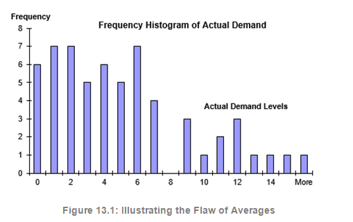
Imagine that you collect 5-years’ worth of historical demand levels and write down the demand quantity on a golf ball for each month. Throw all 60 golf balls into a large basket and mix the basket randomly. Pick a golf ball out at random and write down its value on a piece of paper, then replace the ball in the basket and mix the basket again. Do this 60 times, and calculate the average. This process is a single grouped trial. Perform this entire process several thousand times, with replacement. The distribution of these thousands of averages represents the outcome of the simulation forecast. The expected value of the simulation is simply the average value of these thousands of averages. Figure 13.2 shows an example of the distribution stemming from a nonparametric simulation. As you can see, the optimal inventory rate that minimizes carrying costs is nine units, far from the average value of five units previously calculated in Figure 13.1.
Clearly, each approach has its merits and disadvantages. Nonparametric simulation, which can be easily applied using Risk Simulator’s nonparametric custom distribution, uses historical data to tell the story and to predict the future. Parametric simulation, however, forces the simulated outcomes to follow well-behaving distributions, which is desirable in most cases. Instead of having to worry about cleaning up any messy data (e.g., outliers and nonsensical values) as is required for nonparametric simulation, parametric simulation starts fresh every time.
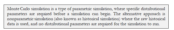
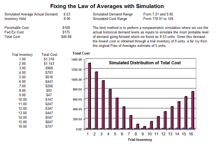
Figure 13.2: A Fix for the Flaw of Averages