File Name: Simulation – Demand Curve and Elasticity Estimation
Location: Modeling Toolkit | Risk Simulator | Demand Curve and Elasticity Estimation
Brief Description: Illustrates how to use Risk Simulator for determining the price elasticity of demand for a historical set of price and quantity sold data for linear and nonlinear functions
Requirements: Modeling Toolkit, Risk Simulator
This model illustrates how the price elasticity of demand can be computed from historical sale price and quantity sold. The resulting elasticity measure is then used in the Optimization – Optimal Pricing with Elasticity model to determine the optimal prices to charge for a product in order to maximize total revenues.
This model is used to find the optimal pricing levels that will maximize revenues through the use of historical elasticity levels. The price elasticity of demand is a basic concept in microeconomics, which can be briefly described as the percentage change of quantity divided by the percentage change in prices. For example, if, in response to a 10% fall in the price of a good, the quantity demanded increases by 20%, the price elasticity of demand would be 20% / (−10%) = −2. In general, a fall in the price of a good is expected to increase the quantity demanded, so the price elasticity of demand is negative. In some literature, the negative sign is omitted for simplicity (denoting only the absolute value of the elasticity).
We can model this elasticity in several ways, including the point elasticity by taking the first derivative of the inverse of the demand function and multiplying it by the ratio of price to quantity at a particular point on the demand curve:
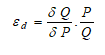
where ε is the price elasticity of demand, P is price, and Q is the quantity demanded.
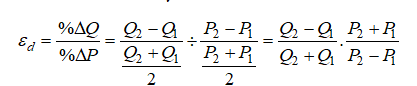
Instead of using instantaneous point elasticities, this example uses the discrete version, where we define elasticity as:
To further simplify things, we assume that in a group of hotel rooms, cruise ship tickets, airline tickets, or any other products with various categories (e.g., standard room, executive room, suite, etc.), there is an average price and average quantity of units sold per period. Therefore, we can further simplify the equation to:
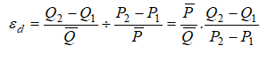
where we now use the average price and average quantity demanded values ![]()
If we have in each category the average price and average quantity sold such as in the model, we can compute the expected quantity sold given a new price if we have the historical elasticity of demand values.
The example model in Figure 139.1 shows how a nonlinear price-quantity relationship yields a static and unchanging elasticity, whereas a linear price-quantity relationship typically yields changing elasticities over the entire price range. Nonlinear extrapolation and linear regression are run to determine the linearity and nonlinearity of the prices. For the nonlinear relationship, a loglinear regression can be run to determine the single elasticity value (Figure 139.2). Elasticities of a linear relationship have to be determined at every price level using the aforementioned equations.
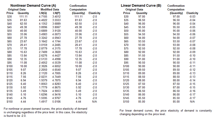
Figure 139.1: Nonlinear demand curve with static elasticity versus linear demand curve with changing elasticity
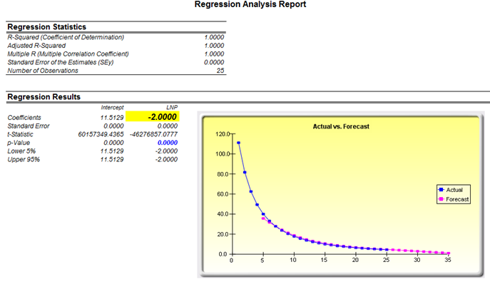
Figure 139.2: Nonlinear demand curve’s elasticity estimated using a nonlinear regression