In the Advanced Custom Optimization tab (see Figures 8.3–8.7), you can create and solve your own optimization models. Knowledge of optimization modeling is required to set up your own models, but you can click on Load Example and select a sample model to run. You can use these sample models to learn how the Optimization routines can be set up. Click Run when done to execute the optimization routines and algorithms. The calculated results and charts will be presented on completion.
When setting up your own optimization model, we recommend going from one tab to another, starting with the Method (static, dynamic, or stochastic optimization); setting up the Decision Variables, Constraints, and Statistics (applicable only if simulation inputs have first been set up, and if dynamic or stochastic optimization is run); and setting the Objective function.
Method: Static Optimization
As far as the optimization process is concerned, PEAT’s Advanced Custom Optimization can be used to run a Static Optimization, that is, an optimization that is run on a static model, where no simulations are run. In other words, all the inputs in the model are static and unchanging. This optimization type is applicable when the model is assumed to be known and no uncertainties exist. Also, a discrete optimization can be first run to determine the optimal portfolio and its corresponding optimal allocation of decision variables before more advanced optimization procedures are applied. For instance, before running a stochastic optimization problem, a discrete optimization is first run to determine if there exist solutions to the optimization problem before a more protracted analysis is performed.
Method: Dynamic Optimization
Next, Dynamic Optimization is applied when Monte Carlo simulation is used together with optimization. Another name for such a procedure is Simulation-Optimization. That is, a simulation is first run, then the results of the simulation are applied back into the model, and then an optimization is applied to the simulated values. In other words, a simulation is run for N trials, and then an optimization process is run for M iterations until the optimal results are obtained, or an infeasible set is found. That is, using PEAT’s optimization module, you can choose which forecast and assumption statistics to use and replace in the model after the simulation is run. Then, these forecast statistics can be applied in the optimization process. This approach is useful when you have a large model with many interacting assumptions and forecasts, and when some of the forecast statistics are required in the optimization. For example, if the standard deviation of an assumption or forecast is required in the optimization model (e.g., computing the Sharpe ratio in asset allocation and optimization problems where we have mean divided by standard deviation of the portfolio), then this approach should be used.
Method: Stochastic Optimization
The Stochastic Optimization process, in contrast, is similar to the dynamic optimization procedure with the exception that the entire dynamic optimization process is repeated T times. That is, a simulation with N trials is run, and then an optimization is run with M iterations to obtain the optimal results. Then the process is replicated T times. The results will be a forecast chart of each decision variable with T values. In other words, a simulation is run and the forecast or assumption statistics are used in the optimization model to find the optimal allocation of decision variables. Then, another simulation is run, generating different forecast statistics, and these new updated values are then optimized, and so forth. Hence, the final decision variables will each have their own forecast chart, indicating the range of the optimal decision variables. For instance, instead of obtaining single-point estimates in the dynamic optimization procedure, you can now obtain a distribution of the decision variables and, hence, a range of optimal values for each decision variable, also known as a stochastic optimization.
TIPS on Optimization Method
- You should always run a Static Optimization prior to running any of the more advanced methods to test if the setup of your model is correct.
- The Dynamic Optimization and Stochastic Optimization must first have simulation assumptions That is, both of the approaches require Monte Carlo Risk Simulation to be run prior to starting the optimization routines.
Decision Variables
Decision variables are quantities over which you have control, for example, the amount of a product to make, the number of dollars to allocate among different investments, or which projects to select from among a limited set. As an example, portfolio optimization analysis includes a go or no-go decision on particular projects. In addition, the dollar or percentage budget allocation across multiple projects also can be structured as decision variables.
TIPS on Optimization Decision Variables
- Click Add to add a new Decision Variable. You can also Change, Delete, or Duplicate an existing decision variable.
- Decision Variables can be set as Continuous (with lower and upper bounds), Integers (with lower and upper bounds), Binary (0 or 1), or a Discrete Range.
- The list of available variables is shown in the data grid, complete with their assumptions.
Constraints
Constraints describe relationships among decision variables that restrict the values of the decision variables. For example, a constraint might ensure that the total amount of money allocated among various investments cannot exceed a specified amount or, at most, one project from a certain group can be selected; budget, timing, minimum returns, or risk tolerance levels are other examples of constraints.
TIPS on Optimization Constraints
- Click Add to add a new Constraint. You can also Change or Delete an existing constraint.
- When you add a new constraint, the list of available Variables will be shown. Simply double-click on a desired variable and its variable syntax will be added to the Expression window. For example, double-clicking on a variable named “Return1” will create a syntax variable “$(Return1)$” in the window.
- Enter your own constraint equation. For example, the following is a constraint:
$(Asset1)$+$(Asset2)$+$(Asset3)$+$(Asset4)$=1, where the sum of all four decision variables must add up to 1.
- Keep adding as many constraints as you need but be aware that the higher the number of constraints, the longer the optimization will take, and the higher the probability of your making an error or creating nonbinding constraints or having constraints that violate another existing constraint (thereby introducing an error in your model).
Statistics
The Statistics subtab will be populated only if there are simulation assumptions set up.
TIPS on Optimization Statistics
- The Statistics window will only be populated if you have previously defined simulation assumptions available.
- If there are simulation assumptions set up, you can run Dynamic Optimization or Stochastic Optimization; otherwise, you are restricted to running only Static Optimizations.
- In the window, you can click on the statistics individually to obtain a drop-down list. Here you can select the statistic to apply in the optimization The default is to return the Mean from the Monte Carlo Risk Simulation and replace the variable with the chosen statistic (in this case the average value), and Optimization will then be executed based on this statistic.
Objective
Objectives give a mathematical representation of the model’s desired outcome, such as maximizing profit or minimizing cost, in terms of the decision variables. In financial analysis, for example, the objective may be to maximize returns while minimizing risks (maximizing the Sharpe’s ratio or returns-to-risk ratio).
TIPS on Optimization Objective
- You can enter your own customized Objective in the function window. The list of available variables is shown in the Variables window on the right. This list includes predefined decision variables and simulation assumptions.
- An example of an objective function equation looks something like:($(Asset1)$*$(AS_Return1)$+$(Asset2)$*$(AS_Return2)$+$(Asset3)$*$(AS_Return3)$+$(Asset4)$*$(AS_Return4)$
)/sqrt($(AS_Risk1)$**2*$(Asset1)$**2+$(AS_Risk2)$**2*$(Asset2)$**2+$(AS_Risk3)$**2*$(Asset3)$**2+$(AS_Risk4
)$**2*$(Asset4)$**2)
- You can use some of the most common math operators such as +, -, *, /, **, where the latter is the function for “raised to the power of.”
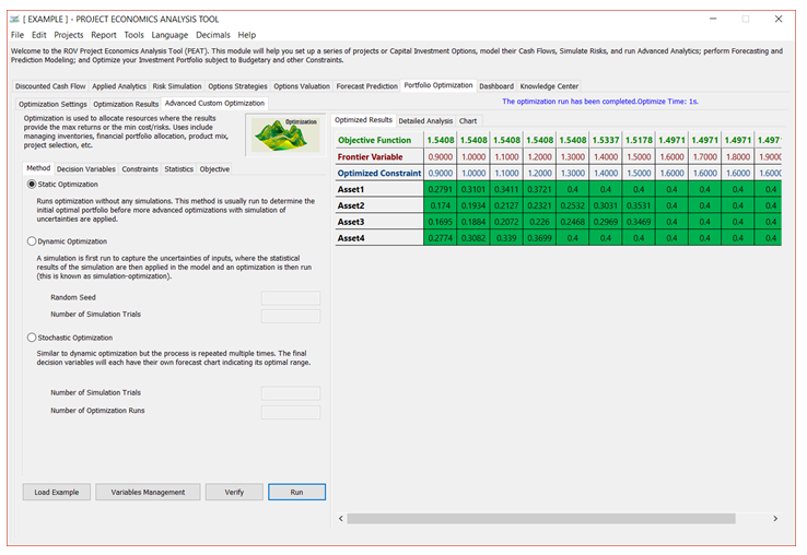
Figure 8.3 – Portfolio Optimization: Method
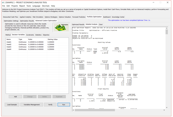
Figure 8.4 – Portfolio Optimization: Decision Variables
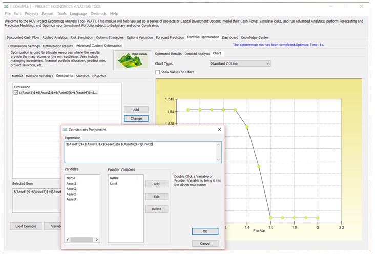
Figure 8.5 – Portfolio Optimization: Constraints
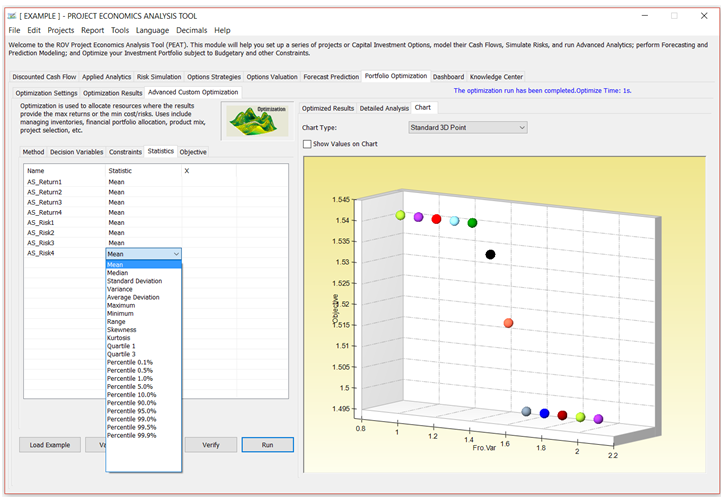
Figure 8.6 – Portfolio Optimization: Statistics
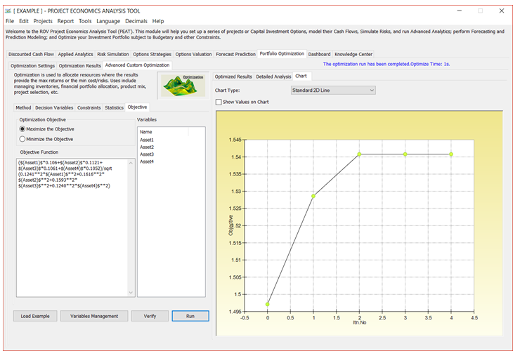
Figure 8.7 – Portfolio Optimization: Objective