- Related AI/ML Methods: Normit Probit Binary Classification, Multivariate Discriminant Analysis
- Related Traditional Methods: Generalized Linear Models, Logit, Probit, Tobit
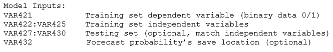
Limited dependent variables techniques are used to forecast the probability of something occurring given some independent variables (e.g., predicting if a credit line will default given the obligor’s characteristics such as age, salary, credit card debt levels; or the probability a patient will have lung cancer based on age and number of cigarettes smoked annually, and so forth). The dependent variable is limited (i.e., binary 1 and 0 for default/cancer, or limited to integer values 1, 2, 3, etc.). Traditional regression analysis will not work as the predicted probability is usually less than 0 or greater than 1, and many of the required regression assumptions are violated (e.g., independence and normality of the errors). We also have a vector of independent variable regressors, X, which are assumed to influence the outcome, Y. A typical ordinary least squares regression approach is invalid because the regression errors are heteroskedastic and non-normal, and the resulting estimated probability estimates will return nonsensical values of above 1 or below 0. This analysis handles these problems using an iterative optimization routine to maximize a log-likelihood function when the dependent variables are limited.
The AI Machine Learning Logistic Binary Classification (Figure 9.77) regression is used for predicting the probability of occurrence of an event by fitting data to a logistic curve. It is a Generalized Linear Model used for binomial regression, and, like many forms of regression analysis, it makes use of several predictor variables that may be either numerical or categorical. Maximum Likelihood Estimation (MLE) is applied in a binary multivariate logistic analysis to determine the expected probability of success of belonging to a certain group.
The estimated coefficients for the Logistic model are the logarithmic odds ratios and cannot be interpreted directly as probabilities. A quick computation is first required. Specifically, the Logit model is defined as Estimated ![]() or (
or (![]() ) using
) using ![]() or, conversely,
or, conversely, ![]() , and the coefficients
, and the coefficients ![]() are the log odds ratios. So, taking the antilog or
are the log odds ratios. So, taking the antilog or ![]() we obtain the odds ratio of
we obtain the odds ratio of ![]() . This means that with an increase in a unit of
. This means that with an increase in a unit of ![]() , the log odds ratio increases by this amount. Finally, the rate of change in the probability is
, the log odds ratio increases by this amount. Finally, the rate of change in the probability is ![]() . The standard error measures how accurate the predicted coefficients are, and the t-statistics are the ratios of each predicted coefficient to its standard error and are used in the typical regression hypothesis test of the significance of each estimated parameter. To estimate the probability of success of belonging to a certain group (e.g., predicting if a smoker will develop chest complications given the amount smoked per year), simply compute the estimated
. The standard error measures how accurate the predicted coefficients are, and the t-statistics are the ratios of each predicted coefficient to its standard error and are used in the typical regression hypothesis test of the significance of each estimated parameter. To estimate the probability of success of belonging to a certain group (e.g., predicting if a smoker will develop chest complications given the amount smoked per year), simply compute the estimated ![]() value using the MLE coefficients. For example, if the model is
value using the MLE coefficients. For example, if the model is ![]() , then for someone smoking 100 packs per year,
, then for someone smoking 100 packs per year,![]() Next, compute the inverse antilog of the odds ratio by doing:
Next, compute the inverse antilog of the odds ratio by doing: ![]() . So, such a person has an 83.20% chance of developing some chest complications in his or her lifetime.
. So, such a person has an 83.20% chance of developing some chest complications in his or her lifetime.
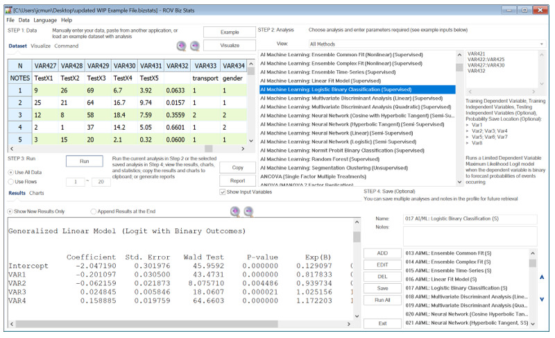
Figure 9.77: AI/ML Logistic Binary Classification (Supervised)
The results interpretation is similar to that of a standard multiple regression, with the exception of computing the probability. For example, in Figure 9.77, the first row of the testing variable’s data points are 9, 26, 69, 6.7, which means that the ![]() .
.
Next, we can compute the inverse antilog of the odds ratio by doing: ![]() . The remaining rows are similarly computed.
. The remaining rows are similarly computed.
In addition, the results also return a confusion matrix, which lists the true responses based on the training set’s dependent variable and the predicted responses. The matrix shows the various positivity and recall rates as well as the specificity, prevalence of false positives, and false negatives. True Positive (TP) is where the actual is 1 and the predicted is 1, and we see that 67.37% of the dataset was predicted correctly as a true positive. The same interpretation applies to False Negatives (FN), False Positives (FP), and True Negatives (TN).
In addition, Positive Sensitivity Recall is TP/(TP+FN) and it measures the ability to predict positive outcomes. Negative Specificity is TN/(TN+FP) and it measures the ability to predict negative outcomes. Event Prevalence is the amount of Actual Y=1 and it measures the positive outcomes in the original data. False Positives is FP/(FP+TP) or Type I error. False Negatives is FN/(FN+TN) or Type II error. Positive Precision is TP/(TP+FP) and it measures the accuracy of a predicted positive outcome. Negative Precision is TN/(TN+FN) and it measures the accuracy of a predicted negative outcome. The Accuracy of the overall prediction is the % of TP and TN.
Finally, the results show the Receiver Operating Characteristic (ROC) curve (Figure 9.78). It plots the Positive Sensitivity Rate against the Negative Specificity, where the area under the curve (AUC) is another measure of the accuracy of the classification model. The ROC plots the model’s performance at all classification thresholds. AUC ranges from 0%–100%, where 100% indicates a perfect fit. The ROC is available by clicking on the Charts subtab in BizStats while the AUC result is shown as one of the accuracy measures in the Confusion Matrix section.
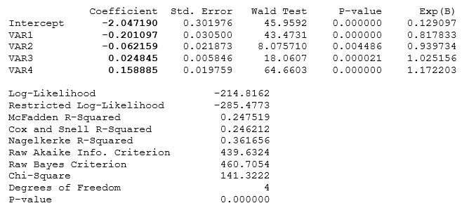
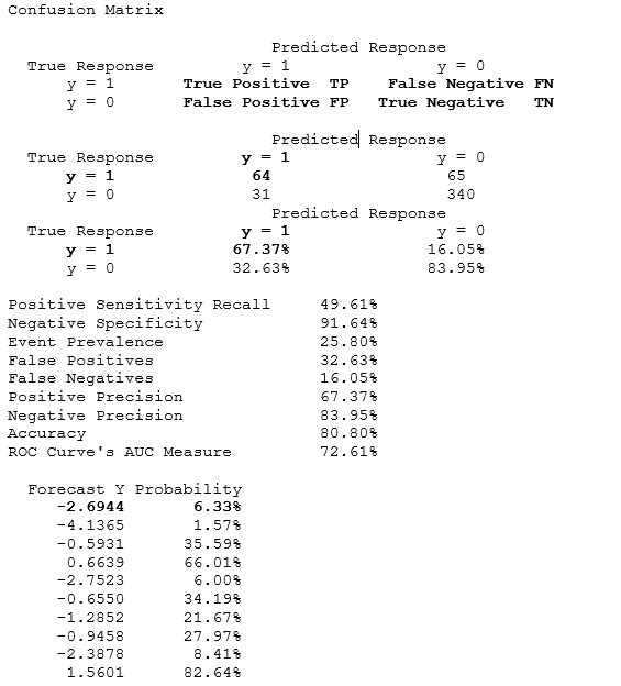
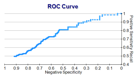
Figure 9.78: ROC and AUC