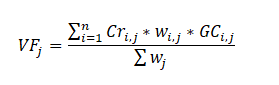
The Vulnerability Factor (VF) is associated with a set of controls (Cri,j), based on international standards or internal rules that must be fulfilled to reduce the Risk Element (REj)to a level of residual risk. Each control (Cri,j) by REj selected should be associated with a weight (wi,j) equal to one, two, or four, depending on the degree of importance attached to it. The use of weights allows us to distinguish between controls that are more difficult to be implemented or which would have a much greater impact on risk mitigation. Our suggestion is to rank the controls by the degree of impact: minor impact should be classified as having a weight identical to unity; the average impact, a weight equal to 2 (two); and, finally, if any, high impact with a weight of 4 (four), providing a sense of geometric growth. After an audit, controls may have different degrees of conformity (GCi,j), namely, implemented (0%), partially implemented (50%), and non-deployed (100%). The REj audited Vulnerability Factor (VFi,j) is calculated using the following formula:
Case Illustration
Figure 4.5 illustrates a manual computation of several sample Risk Elements, their respective Risk Controls, Weights, Vulnerability %, and the computed Vulnerability Factor (%VF) and Degree of Mitigation (%DM). It also shows a screenshot of the PEAT ERM Risk Register tab showing how these assumptions can be entered and the subsequent simple steps required to set up the ERM Risk Register.
Explanation Details
- A Risk Register comprises multiple Risk Elements. Figure 4.6’s PEAT ERM shows three sample saved Risk Registers, with the highlighted Risk Register being actively edited (e.g., Risk Register Project DGS728 is currently selected).
- A Risk Element means an actual or anticipated risk. In the table, we see there are n Risk Elements in a single Risk Register. The first Risk Element example is a catastrophic fire risk event at one of the plants or utility facilities, another risk is employee accidents at the plants (Risk Element 2), and so forth, ending with legal risks (Risk Element N).
- In the first Risk Element, the catastrophic fire, let’s say, for illustration purposes, there are three problems relating to this fire: destruction and loss of assets (Assets), loss of production and output (Production), and loss of human productivity (Productivity).
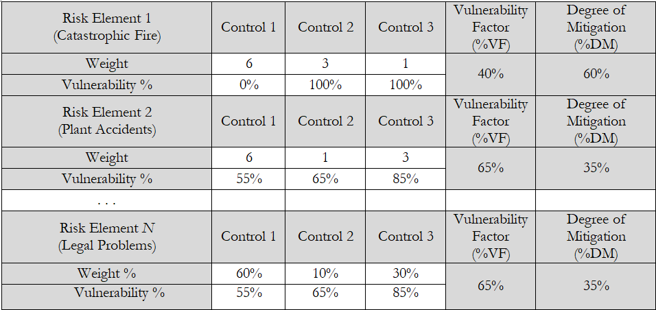
Figure 4.5: PEAT ERM Risk Register
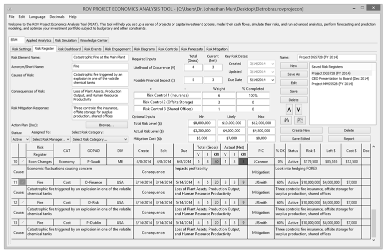
Figure 4.6: PEAT ERM Risk Register
- Each problem is mitigated by a control. Control 1 mitigates losses in Assets by purchasing fire insurance; Control 2 mitigates losses in Production by installing capacitors and storage areas in a different off-site location that can store excess production and handle demand for the next 90 days after a catastrophic fire; and Control 3 mitigates Productivity losses by initiating a joint venture with a partner company to house all the employees at a temporary workplace while at the same time migrating all IT systems to a cloud-based environment for instant restoration of proprietary data such that employees can get back to work almost immediately.
- Let’s further assume a simple scenario involving Risk Element 1 where the estimated total and complete catastrophic fire event will mean a loss of $6M in Assets, $3M in Production, and $1M in Productivity. These amounts were obtained through an audit by the risk personnel by performing inventory of the assets, financial analysis of production rates and loss revenues, and human resource estimations. Using these estimates, we can enter the relevant weights, either as numerical values or percentages. For instance, Control 1 has a weight of 6, Control 2 has a weight of 3, and Control 3 has a weight of 1, commensurate with the total gross risk covered and impact mitigated by each control for this single Risk Element. Of course, each company may have its own paradigm in setting the weights, as long as it is consistent throughout its ERM In this simple example we look at weighting the risk-reduction impact, whereas different organizations who do not have such impact numbers may similarly use degree of difficulty to execute the control, complication, or cost to implement (in which case the weights will be different than in the example above).
- Furthering our example, let’s say that Control 1 (fire insurance) is very simple to execute and coverage was already purchased for the full amount of the Assets, which means that the % Mitigation Completed (%M) is 100% or, alternatively, % Vulnerability (%V) is 0%. Controls 2 and 3 are more difficult to complete and take time and money, and, as of right now, they are 0% completed (0% mitigated or 100% vulnerable if a fire occurs).
- As a side note, %M and %V are complementary to each other (i.e., 1 – %V = %D), and expressing either vulnerability or degree of mitigation is a matter of preference (%M takes a more optimistic point of view whereas %V takes a more pessimistic point of view, but converting from one measure to another is very simple as described).
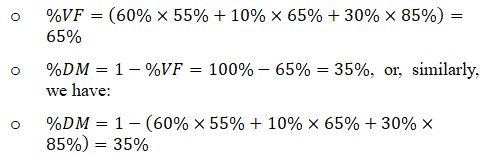
- See Figure 4.5 for Risk Element 2 (employee accidents at the plant) for another sample set of inputs. Finally, Risk Element N intentionally showcases the same weighting levels but here a percentage weight is used instead. Therefore, instead of a numerical weight of 6, 1, 3 (which sums to 10), we can alternatively input these as 60%, 10%, and 30% (this is equivalent to 6/10, 1/10, and 3/10). This is a user preference and can be set in PEAT ERM’s Global Settings tab.
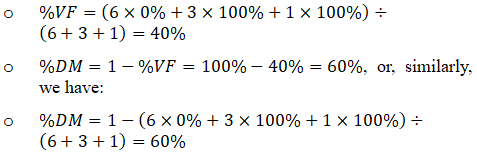
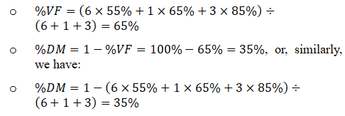
- Then, the PEAT ERM module automatically computes the Vulnerability Factor (%VF) and the Degree of Mitigation (%DM) for each of the Risk The following shows their respective calculations:
Risk Element 1: Catastrophic Fire.
Risk Element 2: Plant Accidents.
Risk Element N: Legal Issues. In this example, we use % weights instead of numerical.
As a side note, the numerical weight can take on any positive integer and does not have any further restrictions, whereas the % weight each needs to be between 0% and 100%, and the total weights for each Risk Element must sum to 100%.
- The monetary Gross Risk for Risk Element 1 (catastrophic fire) is, of course, $6M + $3M + $1M = $10M. And in the example above, we see that only Control 1 (fire insurance) was 100% mitigated (0% vulnerable). This means the entire $6M has been mitigated and the risk no longer exists, at least financially speaking. Thus, the Remaining or Residual Risk is $3M + $1M = $4M. Alternatively, we can compute the Residual Risk = Gross Risk × % Vulnerability Factor. Of course, this is the same as saying Residual Risk = Gross Risk × (1-% Degree of Mitigation). That is, we can compute Residual Risk = $10M × 40% = $10M × (1-60%) = $4M. This $4M is the Remaining or Residual Risk or the risk that remains after the Risk Controls are in place. As a side note, COSO requirements specifically state to use Impact and Likelihood measures and define Gross Risk as Inherent Risk, and Residual Risk as the remaining risks after management executes whatever controls they have executed. (See Chapter 3 for specifications of how PEAT complies with Basel III/IV, ISO 31000:2009, and COSO global standards.) Regardless of the definitions used in the example here, clearly, different companies have different paradigms; the important thing is to be consistent in defining them. If we compute the Remaining Risk in the example above, the user has the option to change the name “Residual Risk” to something like “Actual or Remaining Risk” in the PEAT ERM’s Global Settings tab to avoid any confusion.
Procedures
The following shows how to use PEAT ERM to input Risk Elements and Risk Controls into a Risk Register (Figure 4.6):
- Step 1: In the relevant Risk Register, users can input new Risk Elements in the data grid or edit an existing Risk Element (click on the pencil icon in the data grid for the relevant row to edit). Each Risk Element is shown as a new row in the Risk Register’s data grid.
- Step 2: Enter the Risk Controls, Weight, and % Mitigation Completed for each control item (weights can be entered as integers or percentages depending on user settings in the Global Settings tab). The % Degree of Mitigation is automatically computed and shown in the data grid under the %OK column.
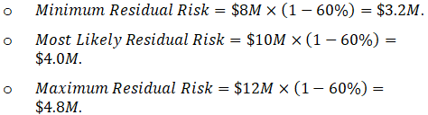
- Step 3: Users can optionally enter the monetary Gross Risk amounts if required and known, as well as a spread that will be used later in running Monte Carlo risk simulations. For instance, enter $8M, $10M, and $12M, where the most likely Gross Risk is $10M as illustrated in this example (the sum of the Assets, Production, and Productivity).
- Step 4: Users can then optionally enter the monetary Residual Risk amounts if required. This is very simple to enter: simply take the Gross Risk amounts and multiply by (1 – %DM). In this example, the Residual Risk spreads will be:
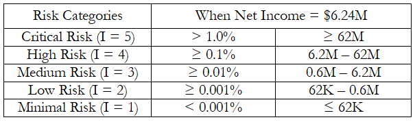
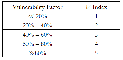
- Step 5: Depending on whether the user has previously selected the Impact and Vulnerability or the Impact and Likelihood settings for the Risk Matrix in the Global Settings tab of PEAT ERM, users can either use the $4M computed Actual Risk or Residual Risk amount or the %OK (i.e., % Vulnerability Factor for the Risk Element after performing the weighted average computation of the various Risk Controls), or they can use their own specified categories and enter either the V or I For example, the following is a simple example of company-specific V and I values, which can be tied to net income, revenues, or other financial metrics and are obviously unique to each company and may change over time. These categorizations will be decided by the company’s risk committee (the example below is for a 5 × 5 risk matrix):
- Step 6: Continue adding more Risk Elements in the Risk Register, perform the tornado and scenario analyses and the simulation analysis, and run the various Risk Dashboard reports.