One very powerful tool in Monte Carlo simulation is that of precision control. For instance, how many trials are considered sufficient to run in a complex model? Precision control takes the guesswork out of estimating the relevant number of trials by allowing the simulation to stop if the level of prespecified precision is reached.
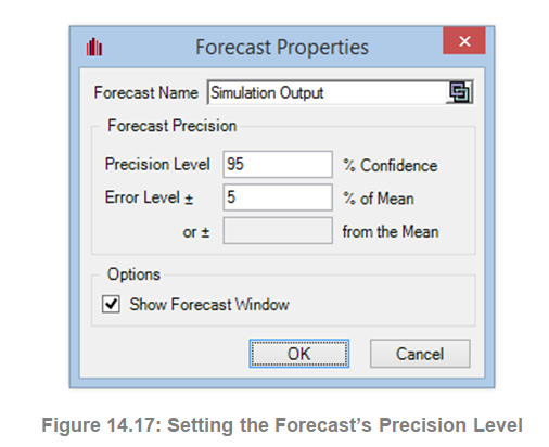
The precision control functionality lets you set how precise you want your forecast to be. Generally speaking, as more trials are calculated, the confidence interval narrows, and the statistics become more accurate. The precision control feature in Risk Simulator uses the characteristic of confidence intervals to determine when a specified accuracy of a statistic has been reached. For each forecast, you can specify the specific confidence interval for the precision level (Figure 14.17). If the error precision is achieved within the number of trials you set, the simulation will run as usual, otherwise, you will be informed that additional simulation trials are required to meet the more stringent required error precision.
Make sure that you do not confuse three very different terms: error, precision, and confidence. Although they sound similar, the concepts are significantly different from one another. A simple illustration is in order. Suppose you are a taco shell manufacturer and are interested in finding out how many broken taco shells there are on average in a box of 100 shells. One way to do this is to collect a sample of pre packaged boxes of 100 taco shells, open them, and count how many of them are actually broken. You manufacture 1 million boxes a year (this is your population), but you randomly open only 10 boxes (this is your sample size, also known as your number of trials in a simulation). The number of broken shells in each box is as follows: 24, 22, 4, 15, 33, 32, 4, 1, 45, and 2. The calculated average number of broken shells is 18.2. Based on these 10 samples or trials, the average is 18.2 units, while based on the sample, the 80% confidence interval is between 2 and 33 units (that is, 80% of the time, the number of broken shells is between 2 and 33 based on this sample size or the number of trials run). However, how sure are you that 18.2 is the correct average? Are 10 trials sufficient to establish this?
The confidence interval between 2 and 33 is too wide and too variable. Suppose you require a more accurate average value where the error is ±2 taco shells 90% of the time––this means that if you open all 1 million boxes manufactured in a year, 900,000 of these boxes will have broken taco shells on average at some mean unit ±2 tacos. How many more taco shell boxes would you then need to sample (or trials run) to obtain this level of precision? Here, the “2 tacos” is the error level while the 90% is the level of precision. If sufficient numbers of trials are run, then the 90% confidence interval will be identical to the 90% precision level, where a more precise measure of the average is obtained such that 90% of the time, the error, and, hence, the confidence will be ±2 tacos. As an example, say the average is 20 units, then the 90% confidence interval will be between 18 and 22 units, where this interval is precise 90% of the time, where in opening all 1 million boxes, 900,000 of them will have between 18 and 22 broken tacos. The number of trials required to hit this precision is based on the sampling error equation of
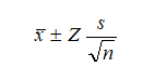
where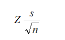
is the error of 2 tacos, ![]() is the sample average, Z is the standard-normal Z-score obtained from the 90% precision level, s is the sample standard deviation, and n is the number of trials required to hit this level of error with the specified precision.
is the sample average, Z is the standard-normal Z-score obtained from the 90% precision level, s is the sample standard deviation, and n is the number of trials required to hit this level of error with the specified precision.
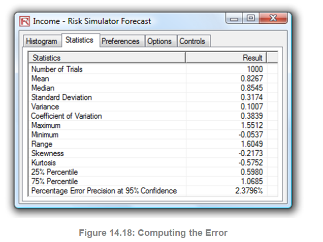
Figures 14.17 and 14.18 illustrate how precision control can be performed on multiple simulated forecasts in Risk Simulator. This feature prevents the user from having to decide how many trials to run in a simulation and eliminates all possibilities of guesswork. Figure 14.17 illustrates the set forecast user interface with a 95% precision level set. The calculated error precision levels of the simulation will be reflected in the last line of the Statistics tab as shown in Figure 14.18.