The Lilliefors test evaluates the null hypothesis of whether the data sample was drawn from a normally distributed population, versus an alternate hypothesis that the data sample is not normally distributed. This test relies on two cumulative frequencies: one derived from the sample dataset and one from a theoretical distribution based on the mean and standard deviation of the sample data. An alternative to this test is the chi-square test for normality. The chi-square test requires more data points to run compared to the Lilliefors test.
H0: The sample is from a Normal Distribution
Ha: The sample is not from a Normal Distribution
In this test, the sample dataset is first arranged in order, from the smallest value to the largest value. Its observed (O) cumulative frequency is calculated and a corresponding cumulative distribution function (CDF) of the normal distribution is computed based on the observed dataset’s mean and standard deviation. The differences D between 0 and CDF are calculated, and the statistic is computed as ![]() Figure 9.35 illustrates a small sample set of five observations with the Lilliefors test administered. The computed D is 0.2782, which is less than the α = 5% significance level threshold of 0.3370, which means we are unable to reject the null hypothesis and conclude that the small sample size is normally distributed. Note that nonparametric methods have less power but are applicable in smaller sample sizes as illustrated in this example. There are other nonparametric approaches in BizStats used for normality tests, which are slightly more powerful than the Lilliefors test:
Figure 9.35 illustrates a small sample set of five observations with the Lilliefors test administered. The computed D is 0.2782, which is less than the α = 5% significance level threshold of 0.3370, which means we are unable to reject the null hypothesis and conclude that the small sample size is normally distributed. Note that nonparametric methods have less power but are applicable in smaller sample sizes as illustrated in this example. There are other nonparametric approaches in BizStats used for normality tests, which are slightly more powerful than the Lilliefors test:
Nonparametric D’Agostino–Pearson Normality Test. The D’Agostino–Pearson test is used to nonparametrically determine if there is near-normality in the dataset. This tests the null hypothesis that the data is normally distributed.
Nonparametric Shapiro–Wilk–Royston Normality Test. The Shapiro–Wilk test for normality uses the Royston algorithm to test the null hypothesis that the data is normally distributed. This test does require more data points to compute than the Lilliefors and D’Agostino–Pearson tests. For example, the small dataset in Figure 9.35 will be insufficient to run this test.
Q-Q Normal Chart. This Quantile-Quantile chart is a normal probability plot, which is a graphical method for comparing a probability distribution with the normal distribution by plotting their quantiles against each other. It only provides a visual inspection of the near normality of your dataset.
However, if a larger dataset is available, it is always better to perform parametric distributional fitting such as those described previously (Kolmogorov–Smirnov, Akaike, Bayes Criterion, Kuiper, and so forth).
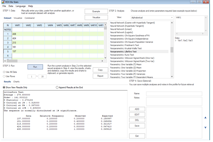
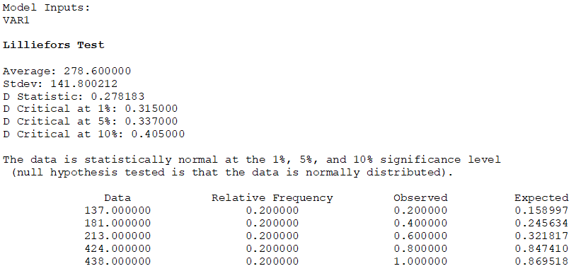
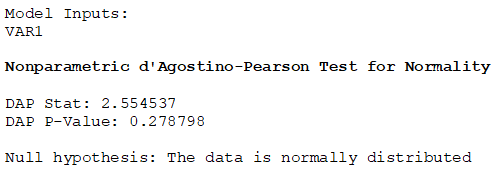
Figure 9.35: Lilliefors Test & D’Agostino–Pearson Test for Normality