The Basics of Correlations
The correlation coefficient is a measure of the strength and direction of the relationship between two variables, and it can take on any values between –1.0 and +1.0. That is, the correlation coefficient can be decomposed into its sign (positive or negative relationship between two variables) and the magnitude or strength of the relationship (the higher the absolute value of the correlation coefficient, the stronger the relationship).
The correlation coefficient can be computed in several ways. The first approach is to manually compute the correlation r of two variables x and y using:
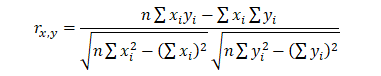
The second approach is to use Excel’s CORREL function. For instance, if the 10 data points for x and y are listed in cells A1:B10, then the Excel function to use is CORREL (A1:A10, B1:B10).
The third approach is to run Risk Simulator’s Analytical Tools | Distributional Fitting | Multi-Variable, and the resulting correlation matrix will be computed and displayed.
It is important to note that correlation does not imply causation. Two completely unrelated random variables might display some correlation, but this does not imply any causation between the two (e.g., sunspot activity and events in the stock market are correlated, but there is no causation between the two).
There are two general types of correlations: parametric and nonparametric correlations. Pearson’s product-moment correlation coefficient is the most common correlation measure and is usually referred to simply as the correlation coefficient. However, Pearson’s correlation is a parametric measure, which means that it requires both correlated variables to have an underlying normal distribution and that the relationship between the variables is linear. When these conditions are violated, which is often the case in Monte Carlo simulation, the nonparametric counterparts become more important. Spearman’s rank correlation and Kendall’s tau are the two nonparametric alternatives. The Spearman correlation is most commonly used and is most appropriate when applied in the context of Monte Carlo simulation—there is no dependence on normal distributions or linearity, meaning that correlations between different variables with different distributions can be applied. In order to compute the Spearman correlation, first rank all the x and y variable values and then apply the Pearson’s correlation computation.
In the case of Risk Simulator, the correlation used is the more robust nonparametric Spearman’s rank correlation. However, to simplify the simulation process, and to be consistent with Excel’s correlation function, the correlation inputs required are the Pearson’s correlation coefficient. Risk Simulator will then apply its own algorithms to convert them into Spearman’s rank correlation, thereby simplifying the process. However, to simplify the user interface, we allow users to enter the more common Pearson’s product-moment correlation (e.g., computed using Excel’s CORREL function), while in the mathematical codes, we convert these simple correlations into Spearman’s rank-based correlations for distributional simulations.
Applying Correlations in Risk Simulator
Correlations can be applied in Risk Simulator in several ways:
- When defining assumptions(Risk Simulator | Set Input Assumption), simply enter the correlations into the correlation matrix grid in the Distribution Gallery of existing assumptions already set up.
- With existing data, run the Multi-Fit tool (Risk Simulator | Analytical Tools | Distributional Fitting | Multiple Variables) to perform distributional fitting and to obtain the correlation matrix between pairwise variables. If a simulation profile exists, the assumptions fitted will automatically contain the relevant correlation values.
- With existing assumptions already set up, you can click on Risk Simulator | Analytical Tools | Edit Correlations to enter the pairwise correlations of all the assumptions directly in one user interface.
Note that the correlation matrix must be positive definite. That is, the correlation must be mathematically valid. For instance, suppose you are trying to correlate three variables: grades of graduate students in a particular year, the number of beers they consume a week, and the number of hours they study a week. One would assume the following relationships:
Grades and Beer: – The more they drink, the lower the grades (no show on exams)
Grades and Study: + The more they study, the higher the grades
Beer and Study: – The more they drink, the less they study (drunk and partying all the time)
However, if you input a negative correlation between Grades and Study, and assuming that the correlation coefficients have high magnitudes, the correlation matrix will be nonpositive definite. It would defy logic, correlation requirements, and matrix mathematics. However, smaller coefficients can sometimes still work even with bad logic. When a nonpositive or bad correlation matrix is entered, Risk Simulator will automatically inform you and adjust these correlations to something that is semi-positive definite while still maintaining the overall structure of the correlation relationship (same signs and relative strengths).
The Effects of Correlations in Monte Carlo Simulation
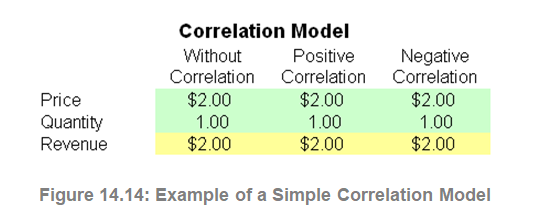
Although the computations required to correlate variables in a simulation are complex, the resulting effects are fairly clear. Figure 14.14 shows a simple correlation model (Risk Simulator | Example Models | Correlation Effects Model). The calculation for revenue is simply price multiplied by quantity. The same model is replicated for no correlations, positive correlation (+0.8), and negative correlation (–0.8) between price and quantity.
The resulting statistics are shown in Figure 14.15. Notice that the standard deviation of the model without correlations is 0.1450, compared to 0.1886 for the positive correlation, and 0.0717 for the negative correlation. That is, for simple models, negative correlations tend to reduce the average spread of the distribution and create a tighter and more concentrated forecast distribution as compared to positive correlations with larger average spreads. However, the mean remains relatively stable. This result implies that correlations do little to change the expected value of projects but can reduce or increase a project’s risk.
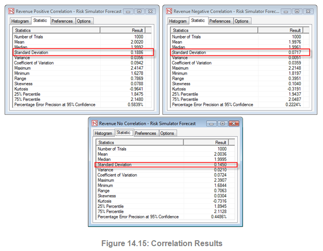
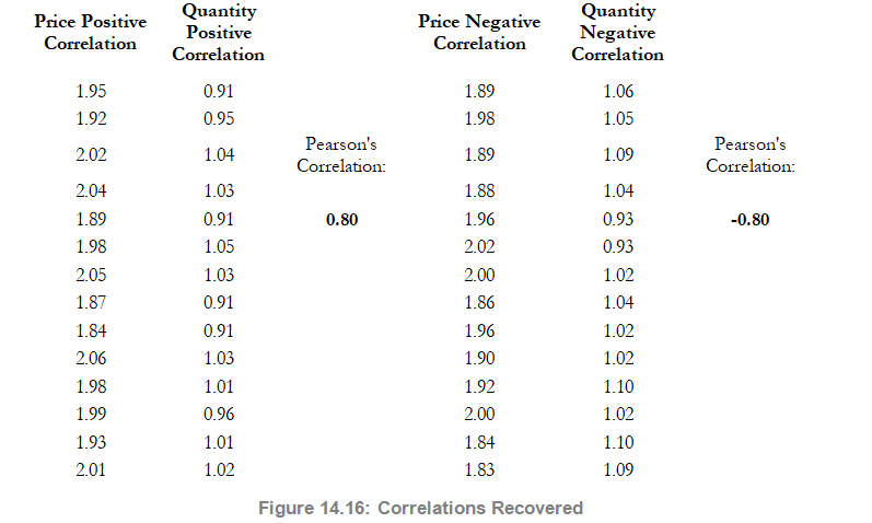
Figure 14.16 illustrates the results after running a simulation, extracting the raw data of the assumptions, and computing the correlations between the variables. The figure shows that the input assumptions are recovered in the simulation. That is, you enter +0.8 and –0.8 correlations, and the resulting simulated values have the same correlations.