File Name: Probability of Default – External Options Model
Location: Modeling Toolkit | Prob of Default | External Options Model (Public Company)
Brief Description: Computes the probability of default and distance to default of a publicly-traded company by decomposing the firm’s book value and market value of liability, assets, and volatility using a simultaneous equations options model with optimization
Requirements: Modeling Toolkit, Risk Simulator
Modeling Toolkit Functions Used: MTMertonDefaultProbabilityII, MTMertonDefaultDistance, MTBlackScholesCall, MTProbabilityDefaultMertonImputedAssetValue, MTProbabilityDefaultMertonImputedAssetVolatility, MTProbabilityDefaultMertonRecoveryRate, MTProbabilityDefaultMertonMVDebt
The probability of default models is a category of models that assesses the likelihood of default by an obligor. These models differ from regular credit scoring models in several ways. First of all, credit scoring models usually are applied to smaller credits (individuals or small businesses) whereas default models are applied more to larger credits (corporations or countries). Credit scoring models are largely statistical, regressing instances of default against various risk indicators, such as an obligor’s income, home renter or owner status, years at a job, educational level, debt to income ratio, and so forth. An example of such a model is seen in the previous chapter, Probability of Default – Empirical Model, where the maximum likelihood approach is used on an advanced econometric regression model. Default models, in contrast, directly model the default process and typically are calibrated to market variables, such as the obligor’s stock price, asset value, debt book value, or credit spread on its bonds. Default models find many applications within financial institutions. They are used to support credit analysis and to find the probability that a firm will default, to value counterparty credit risk limits, or to apply financial engineering techniques in developing credit derivatives or other credit instruments.
This model is used to solve the probability of default of a publicly-traded company with equity and debt holdings and accounting for its volatilities in the market (Figure 114.1). It is currently used by KMV and Moody’s to perform credit risk analysis. This approach assumes that the book value of asset and asset volatility are unknown and solved in the model, and that the company is relatively stable and the growth rate of its assets are stable over time (e.g., not in start-up mode). The model uses several simultaneous equations in options valuation coupled with optimization to obtain the implied underlying asset’s market value and volatility of the asset in order to compute the probability of default and distance to default for the firm.
It is assumed that at this point the reader is well versed in running simulations and optimizations in Risk Simulator. If not, it is suggested that the reader first spends some time on the Simulation – Basic Simulation Model as well as the Continuous Portfolio Optimization chapters before proceeding with the procedures discussed next.
To run this model, enter in the required inputs such as the market value of equity (obtained from market data on the firm’s capitalization, i.e., stock price times number of stocks outstanding), market value of equity (computed in the Volatility or LPVA worksheets in the model), book value of debt and liabilities (the firm’s book value of all debt and liabilities), the risk-free rate (the prevailing country’s risk-free interest rate for the same maturity), the anticipated growth rate of the company (the expected annualized cumulative growth rate of the firm’s assets, estimated using historical data over a long period of time, making this approach more applicable to mature companies rather than start-ups), and the debt maturity (the debt maturity to be analyzed, or enter 1 for the annual default probability). The comparable option parameters are shown in cells G18 to G23. All these comparable inputs are computed except for Asset Value (the market value of assets) and the Volatility of Asset. You will need to input some rough estimates as a starting point so that the analysis can be run. The rule of thumb is to set the volatility of the asset in G22 to be one-fifth to half of the volatility of equity computed in G10, and the market value of assets (G19) to be approximately the sum of the market value of equity and book value of liabilities and debt (G9 and G11).
Then you need to run an optimization in Risk Simulator in order to obtain the desired outputs. To do this, set Asset Value and Volatility of Asset as the decision variables (make them continuous variables with a lower limit of 1% for volatility and $1 for assets, as both these inputs can take on only positive values). Set cell G29 as the objective to minimize as this is the absolute error value. Finally, the constraint is such that cell H33, the implied volatility in the default model, is set to exactly equal the numerical value of the equity volatility in cell G10. Run a static optimization using Risk Simulator.
If the model has a solution, the absolute error value in cell G29 will revert to zero (Figure 114.2). From here, the probability of default (measured in percent) and distance to default (measured in standard deviations) are computed in cells G39 and G41. Then the relevant credit spread required can be determined using the Credit Analysis – Credit Premium model or some other credit spread tables (such as using the Internal Credit Risk Rating model). The simpler alternative is to use Modeling Toolkit’s prebuilt internally optimized functions (we embedded some artificial intelligence integrated with optimization of simultaneous stochastic equations to solve the problem) using
MTProbabilityDefaultMertonImputedAssetValue (cell I21) and
MTProbabilityDefaultMertonImputedAssetVolatility (cell I24)
for obtaining the probability of default (MTProbabilityDefaultMertonII in cell G39).
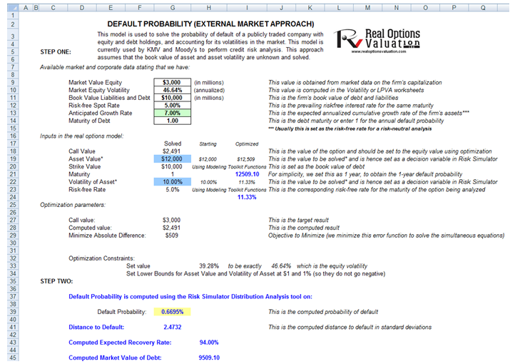
Figure 114.1: Default probability model
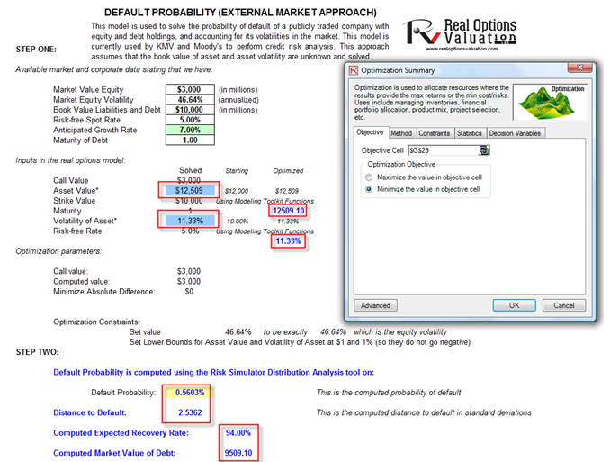
Figure 114.2: Default probability model setup