File Name: Optimization – Continuous Portfolio Allocation
Location: Modeling Toolkit | Optimization | Continuous Portfolio Allocation
Brief Description: Illustrates how to run an optimization on continuous decision variables, and viewing and interpreting optimization results
Requirements: Modeling Toolkit, Risk Simulator
This model shows 10 asset classes with different risk and return characteristics. The idea here is to find the best portfolio allocation such that the portfolio’s bang for the buck or returns to risk ratio is maximized; that is, to allocate 100% of an individual’s investment portfolio among several different asset classes (e.g., different types of mutual funds or investment styles: growth, value, aggressive growth, income, global, index, contrarian, momentum, etc.). In order to run an optimization, several key specifications on the model have to first be identified:
Objective: Maximize Return to Risk Ratio (C18)
Decision Variables: Allocation Weights (E6:E15)
Restrictions on Decision Variables: Minimum and Maximum Required (F6:G15)
Constraints: Portfolio Total Allocation Weights 100% (E17 is set to 100%)
The model shows the 10 asset classes. Each asset class has its own set of annualized returns and risks, measured by annualized volatilities (Figure 94.1). These return and risk measures are annualized values such that they can be consistently compared across different asset classes. Returns are computed using the geometric average of the relative returns, while the risks are computed using the annualized standard deviation of the logarithmic relative historical stock returns approach.
Column E, Allocation Weights, holds the decision variables, which are the variables that need to be tweaked and tested such that the total weight is constrained at 100% (cell E17). Typically, to start the optimization, we will set these cells to a uniform value; in this case, cells E6 to E15 are set at 10% each. In addition, each decision variable may have specific restrictions in its allowed range. In this example, the lower and upper allocations allowed are 5% and 35%, as seen in columns F and G. This setting means that each asset class may have its own allocation boundaries (Figure 94.1).
Next, column H shows the return to risk ratio for each asset class, which is simply the return percentage divided by the risk percentage, where the higher this value, the higher the bang for the buck. The remaining sections of the model show the individual asset class rankings by returns, risk, return to risk ratio, and allocation. In other words, these rankings show at a glance which asset class has the lowest risk or the highest return, and so forth.
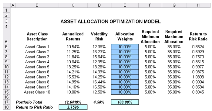
Figure 94.1: Asset allocation optimization model
Running an Optimization
To run this model, simply click on Risk Simulator | Optimization | Run Optimization. Alternatively, for practice, you can try to set up the model again by doing the following (the steps are illustrated in Figure 94.2):
- Start a new profile (Risk Simulator | New Profile) and give it a name.
- Select cell E6 and define the decision variable (Risk Simulator | Optimization | Set Decision, or click on the Set Decision D icon) and make it a Continuous Variable and then link the decision variable’s name and minimum/maximum required to the relevant cells (B6, F6, G6).
- Then use the Risk Simulator Copy on cell E6, select cells E7 to E15, and use Risk Simulator’s Paste (Risk Simulator | Copy Parameter and Risk Simulator | Paste Parameter or use the copy and paste icons). To rerun the optimization, type in 10% for all decision variables. Make sure you do not use Excel’s regular copy and paste functions.
- Next, set up the optimization’s constraints by selecting Risk Simulator | Optimization | Constraints, selecting ADD, and selecting cell E17, and making it (==) equal 100% (for total allocation, and remember to insert the % sign).
- Select cell C18 as the objective to be maximized (Risk Simulator | Optimization | Set Objective).
- Select Risk Simulator | Optimization | Run Optimization. Review the different tabs to make sure that all the required inputs in steps 2–4 are correct.
- You may now select the optimization method of choice and click OK to run the optimization:
- Static Optimization is an optimization that is run on a static model, where no simulations are run. This optimization type is applicable when the model is assumed to be known and no uncertainties exist. Also, a static optimization can be run first to determine the optimal portfolio and its corresponding optimal allocation of decision variables before applying more advanced optimization procedures. For instance, before running a stochastic optimization problem, first run a static optimization to determine if there exist solutions to the optimization problem before performing a more protracted analysis.
- Dynamic Optimization is applied when Monte Carlo simulation is used together with optimization. Another name for such a procedure is Simulation-Optimization. In other words, a simulation is run for N trials, and then an optimization process is run for M iterations until the optimal results are obtained, or an infeasible set is found. That is, using Risk Simulator’s Optimization module, you can choose which forecast and assumption statistics to use and replace in the model after the simulation is run. Then, you can apply these forecast statistics in the optimization process. This approach is useful when you have a large model with many interacting assumptions and forecasts, and when some of the forecast statistics are required in the optimization.
- Stochastic Optimization is similar to the dynamic optimization procedure except that the entire dynamic optimization process is repeated T The results will be a forecast chart of each decision variable with T values. In other words, a simulation is run and the forecast or assumption statistics are used in the optimization model to find the optimal allocation of decision variables. Then another simulation is run, generating different forecast statistics, and these new updated values are optimized, and so forth. Hence, each of the final decision variables will have its own forecast chart, indicating the range of the optimal decision variables. For instance, instead of obtaining single-point estimates in the dynamic optimization procedure, you can now obtain a distribution of the decision variables, and, hence, a range of optimal values for each decision variable, also known as stochastic optimization.
Note: If you are to run either a dynamic or stochastic optimization routine, make sure that you first define the assumptions in the model. That is, make sure that some of the cells in C6:D15 are assumptions. The model setup is illustrated in Figure 94.2.
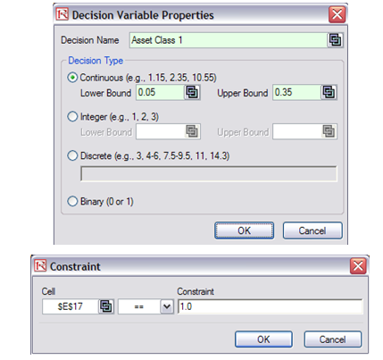
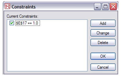
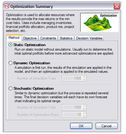
Figure 94.2: Optimization model setup
Results Interpretation
Briefly, the optimization results show the percentage allocation for each asset class (or projects or business lines, etc.) that would maximize the portfolio’s bang-for-the-buck, that is, the allocation that would provide the highest returns subject to the least amount of risk. In other words, for the same amount of risk, what is the highest amount of returns that can be generated, or for the same amount of returns, what is the least amount of risk that can be obtained? See Figure 94.3. This is the concept of the Markowitz efficient portfolio analysis. For a comparable example, see Chapter 100 on the military portfolio model where we also generate the entire efficient frontier model.
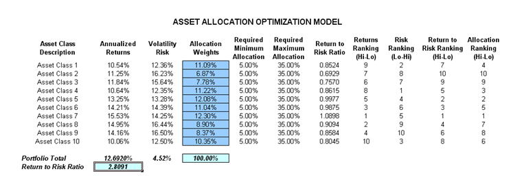
Figure 94.3: Optimization results