Theory
Another powerful simulation tool is distributional fitting; that is, how does an analyst or engineer determine which distribution to use for a particular input variable? What are the relevant distributional parameters? If no historical data exist, then the analyst must make assumptions about the variables in question. One approach is to use the Delphi method, where a group of experts is tasked with estimating the behavior of each variable. For instance, a group of mechanical engineers can be tasked with evaluating the extreme possibilities of a spring coil’s diameter through rigorous experimentation or guesstimates. These values can be used as the variable’s input parameters (e.g., uniform distribution with extreme values between 0.5 and 1.2). When testing is not possible (e.g., market share and revenue growth rate), management can still make estimates of potential outcomes and provide the best-case, most-likely case, and worst-case scenarios, whereupon a triangular or custom distribution can be created.
However, if reliable historical data are available, distributional fitting can be accomplished. Assuming that historical patterns hold and that history tends to repeat itself, then historical data can be used to find the best-fitting distribution with their relevant parameters to better define the variables to be simulated. Figures 15.13 through 15.15 illustrate a distributional-fitting example. The following illustration uses the Data Fitting file in the examples folder.
Procedure
Use the following steps to perform a distributional fitting model:
- Open a spreadsheet with existing data for fitting (e.g., use the Risk Simulator | Example Models | 06 Data Fitting).
- Select the data you wish to fit not including the variable name (data should be in a single column with multiple rows).
- Select Risk Simulator | Analytical Tools | Distributional Fitting (Single-Variable).
- Select the specific distributions you wish to fit to or keep the default where all distributions are selected and click OK (Figure 15.13).
- Review the results of the fit, choose the relevant distribution you want, and click OK (Figure 15.14).
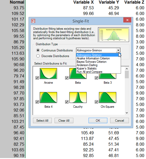
Figure 15.13: Single Variable Distributional Fitting
Results Interpretation
The null hypothesis (H0) being tested is such that the fitted distribution is the same distribution as the population from which the sample data to be fitted come. Thus, if the computed p-value is lower than a critical alpha level (typically 0.10 or 0.05), then the distribution is the wrong distribution. Conversely, the higher the p-value, the better the distribution fits the data. Roughly, you can think of p-value as a percentage explained, that is, if the p-value is 0.9996 (Figure 15.14), then setting a normal distribution with a mean of 100.67 and a standard deviation of 10.40 explains about 99.96% of the variation in the data, indicating an especially good fit. The data was from a 1,000-trial simulation in Risk Simulator based on a normal distribution with a mean of 100 and a standard deviation of 10. Because only 1,000 trials were simulated, the resulting distribution is fairly close to the specified distributional parameters, and in this case, about a 99.96% precision.
Both the results (Figure 15.14) and the report (Figure 15.15) show the test statistic, p-value, theoretical statistics (based on the selected distribution), empirical statistics (based on the raw data), the original data (to maintain a record of the data used), and the assumption complete with the relevant distributional parameters (i.e., if you selected the option to automatically generate assumption and if a simulation profile already exists). The results also rank all the selected distributions and how well they fit the data.
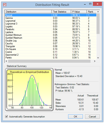
Figure 15.14: Distributional Fitting Result
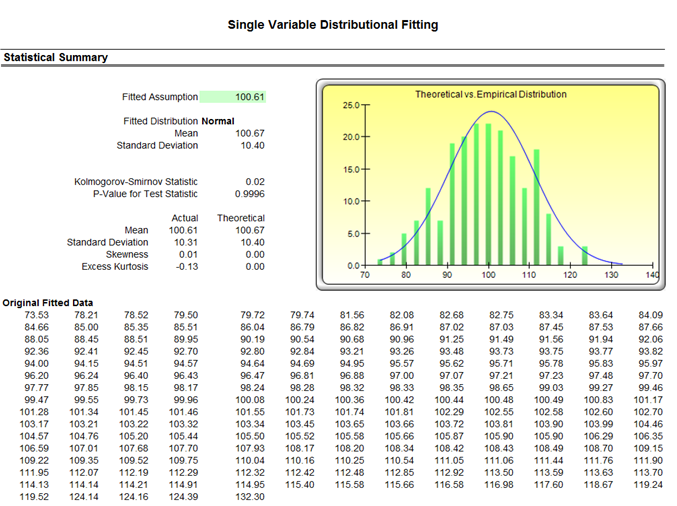
Figure 15.15: Distributional Fitting Report