File Name: Options Analysis – Plain Vanilla Call Options (I-IV) and Plain Vanilla Put Options
Location: Modeling Toolkit | Options Analysis | Plain Vanilla Options (I-IV and Put Options)
Brief Description: Solves plain vanilla call and put option examples using the Real Options SLS software by applying advanced binomial lattices
Requirements: Real Options SLS, Modeling Toolkit
This chapter shows the five plain vanilla call and put options solved using Real Options SLS. These are plain vanillas as they are the simplest call and put options, without any exotic add-ons. A simple European call option is computed in this example using SLS. To follow along, start this example file by first starting the SLS software. Then click on the first icon, Create a New Single Asset Model, and when the single asset SLS opens, click on File | Examples. This is a list of the example files that come with the software for the single asset lattice solver. Start the Plain Vanilla Call Option I example. This example file will be loaded into the SLS software as seen in Figure 110.1. Alternatively, you can start the Modeling Toolkit software, click on Modeling Toolkit in Excel and select Options Analysis, and select the appropriate Options Analysis files. As this chapter uses the Real Options SLS software, it is recommended that readers who are unfamiliar with real options analysis or financial options analysis before proceeding with this chapter.
The starting PV Underlying Asset or starting stock price is $100, and the Implementation Cost or strike price is $100 with a 5-year maturity. The annualized risk-free rate of return is 5%, and the historical, comparable, or future expected annualized volatility is 10%. Click on RUN (or ALT+R) and a 100-step binomial lattice is computed. The results indicate a value of $23.3975 for both the European and American call options. Benchmark values using Black-Scholes and Closed-Form American approximation models as well as standard plain vanilla Binomial American and Binomial European Call and Put Options with 1,000-step binomial lattices are also computed. Notice that only the American and European Options are selected, and the computed results are for these simple plain vanilla American and European call options.
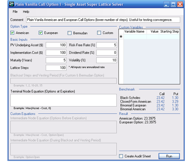
Figure 110.1: SLS Results of simple European and American call options
The benchmark results use both closed-form models (Black-Scholes and Closed-Form Approximation models) and 1,000-step binomial lattices on plain vanilla options. You can change the steps to 1000 in the basic inputs section (or open and use the Plain Vanilla Call Option II example model) to verify that the answers computed are equivalent to the benchmarks as seen in Figure 110.2. Notice that, of course, the values computed for the American and European options are identical to each other and identical to the benchmark values of $23.4187, as it is never optimal to exercise a standard plain vanilla call option early if there are no dividends. Be aware that the higher the lattice step, the longer it takes to compute the results. It is advisable to start with fewer lattice steps to make sure the analysis is robust and then progressively increase lattice steps to check for results convergence. See Chapter 6 of Real Options Analysis, Third Edition (Thomson–Shore, 2016) on convergence criteria on lattices regarding how many lattice steps are required for a robust option valuation. However, as a rule of thumb, the typical convergence occurs between 100 and 1,000 steps.
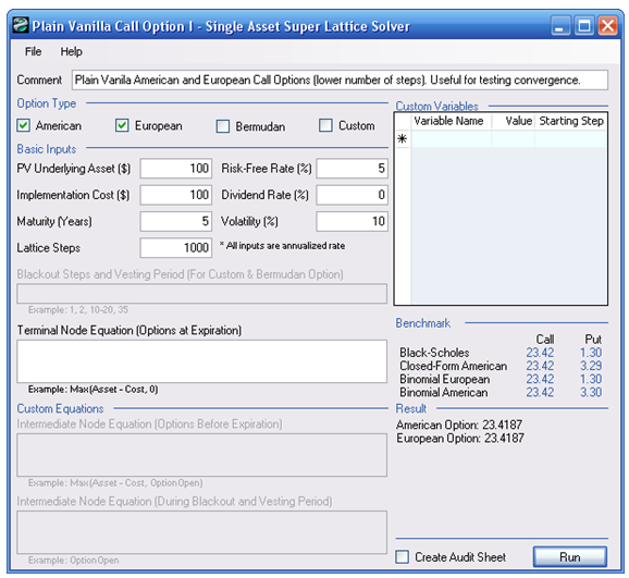
Figure 110.2: SLS comparing results with benchmarks
Alternatively, you can enter Terminal and Intermediate Node Equations for a call option to obtain the same results. Notice that using 100 steps and creating your own Terminal Node Equation of Max(Asset-Cost,0) and Intermediate Node Equation of Max(Asset-Cost,OptionOpen) will yield the same answer. When entering your own equations, make sure to first check Custom Option.
Figure 110.3 illustrates how the analysis is done. The example file used in this example is: Plain Vanilla Call Option III. Notice that the value $23.3975 in Figure 110.3 agrees with the value in Figure 110.1. The Terminal Node Equation is the computation that occurs at maturity, while the Intermediate Node Equation is the computation that occurs at all periods prior to maturity and is computed using backward induction. The term “OptionOpen” (one word, without spaces) represents “keeping the option open,” and is often used in the Intermediate Node Equation when analytically representing the fact that the option is not executed but kept open for possible future execution. Therefore, in Figure 110.3, the Intermediate Node Equation Max(Asset-Cost,OptionOpen) represents the profit maximization decision of either executing the option or leaving it open for possible future execution. In contrast, the Terminal Node Equation of Max(Asset-Cost,0) represents the profit maximization decision at maturity of either executing the option if it is in the money, or allowing it to expire worthless if it is at the money or out of the money.
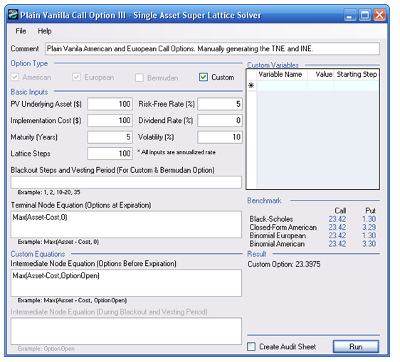
Figure 110.3: Custom equation inputs
In addition, you can create an Audit Worksheet in Excel to view a sample 10-step binomial lattice by checking the box Generate Audit Worksheet. For instance, loading the example file Plain Vanilla Call Option I and selecting the box creates a worksheet as seen in Figure 110.4. Two items on this audit worksheet are noteworthy:
- The audit worksheet generated will show the first 10 steps of the lattice, regardless of how many you enter. That is, if you enter 1000 steps, the first 10 steps will be generated. If a complete lattice is required, simply enter 10 steps in the SLS, and the full 10-step lattice will be generated. The Intermediate Computations and Results are for the Super Lattice, based on the number of lattice steps entered and not based on the 10-step lattice generated. To obtain the Intermediate Computations for 10-step lattices, simply rerun the analysisinputting 10 as the lattice steps. This way, the audit worksheet generated will be for a 10-step lattice, and the results from SLS will now be comparable (Figure 110.5).
- The worksheet only provides values,as it is assumed that the user was the one who entered in the terminal and intermediate node equations, so there is no need to recreate these equations in Excel The user can always reload the SLS file and view the equations or print out the form if required (by clicking on File | Print).
The software also allows you to save or open analysis files. That is, all the inputs in the software will be saved and can be retrieved for future use. The results will not be saved because you may accidentally delete or change an input and the results would no longer be valid. In addition, rerunning the super lattice computations will take only a few seconds. It is always advisable for you to rerun the model when opening an old analysis file.
You may also enter in Blackout Steps, which are the steps on the super lattice that have different behaviors from the terminal or intermediate steps. For instance, you can enter 1000 as the lattice steps and enter 0-400 as the blackout steps, and some Blackout Equation (e.g., OptionOpen). This means that for the first 400 steps, the option holder can only keep the option open. Other examples include entering 1, 3, 5, 10 if these are the lattice steps where blackout periods occur. You will have to calculate the relevant steps within the lattice where the blackout exists. For instance, if the blackout exists in years 1 and 3 on a 10-year, 10-step lattice, then steps 1, 3 will be the blackout dates. This blackout step feature comes in handy when analyzing options with holding periods, vesting periods, or periods where the option cannot be executed. Employee stock options have blackout and vesting periods, and certain contractual real options have periods during which the option cannot be executed (e.g., cooling-off periods, or proof of concept periods).
If equations are entered into the Terminal Node Equation box and American, European, or Bermudan Options are chosen, the Terminal Node Equation entered will be the one used in the super lattice for the terminal nodes. However, for the intermediate nodes, the American option assumes the same Terminal Node Equation plus the ability to keep the option open; the European option assumes that the option can only be kept open and not executed; and the Bermudan option assumes that during the blackout lattice steps, the option will be kept open and cannot be executed. If you also enter the Intermediate Node Equation, first choose the Custom Option. Otherwise, you cannot use the Intermediate Node Equation box. The Custom Option result uses all the equations you have entered in Terminal, Intermediate, and Intermediate with Blackout sections.
The Custom Variables list is where you can add, modify, or delete custom variables, the variables that are required beyond the basic inputs. For instance, when running an abandonment option, you need the salvage value. You can add this in the Custom Variables list and provide it a name (a variable name must be a single word), the appropriate value, and the starting step when this value becomes effective. That is, if you have multiple salvage values (i.e., if salvage values change over time), you can enter the same variable name (e.g., salvage) several times, but each time, its value changes and you can specify when the appropriate salvage value becomes effective. For instance, in a 10-year, 100-step super lattice problem where there are two salvage values––$100 occurring within the first 5 years and increases to $150 at the beginning of Year 6––you can enter two salvage variables with the same name, $100 with a starting step of 0 and $150 with a starting step of 51. Be careful here as Year 6 starts at step 51, not 61. That is, for a 10-year option with a 100-step lattice, we have: Steps 1–10 = Year 1; Steps 11–20 = Year 2; Steps 21–30 = Year 3; Steps 31–40 = Year 4; Steps 41–50 = Year 5; Steps 51–60 = Year 6; Steps 61–70 = Year 7; Steps 71–80 = Year 8; Steps 81–90 = Year 9; and Steps 91–100 = Year 10. Finally, incorporating 0 as a blackout step indicates that the option cannot be executed immediately.
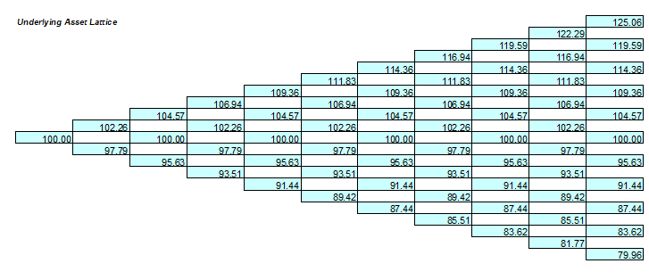
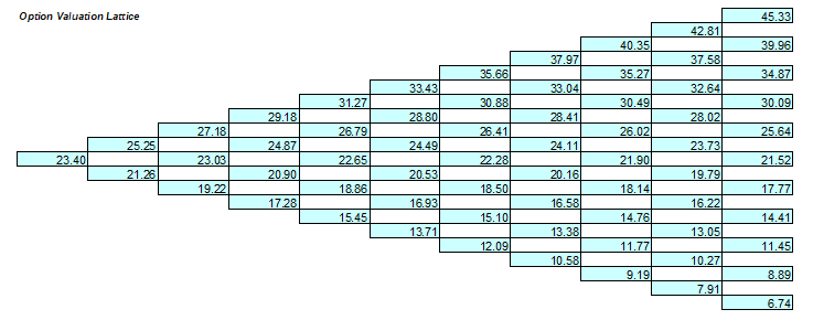
Figure 110.4: SLS-generated audit worksheet
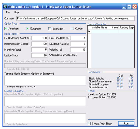
Figure 110.5: SLS results with a 10-step lattice
Finally, using the example file, Plain Vanilla Option IV, we see that when a dividend exists, the American option with its ability for early exercise is worth more than the Bermudan, which has early exercise but blackout periods when it cannot be exercised (e.g., Blackout Steps of 0–95 for a 100-step lattice on a 5-year maturity model means that for the first 4.75 years, the option cannot be executed), which in turn is worth more than the European option, which can be exercised only at expiration (Figure 110.6).
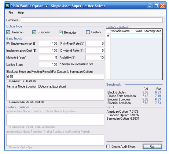
Figure 110.6: American, Bermudan, and European options