The distributional analysis tool is a statistical probability tool in Risk Simulator that is rather useful in a variety of settings. It can be used to compute the probability density function (PDF), which is also called the probability mass function (PMF) for discrete distributions (these terms are used interchangeably), where given some distribution and its parameters, we can determine the probability of occurrence given some outcome x. In addition, the cumulative distribution function (CDF) can be computed, which is the sum of the PDF values up to this x value. Finally, the inverse cumulative distribution function (ICDF) is used to compute the value x given the cumulative probability of occurrence. The following pages provide example uses of PDF, CDF, and ICDF. Also, remember to try some of the exercises at the end of this chapter for more hands-on applications of probability distribution analysis using this tool.
This tool is accessible via Risk Simulator | Analytical Tools | Distributional Analysis. As an example of its use, Figure 15.20 shows the computation of a binomial distribution (i.e., a distribution with two outcomes, such as the tossing of a coin, where the outcome is either Heads or Tails, with some prescribed probability of heads and tails). Suppose we toss a coin two times and set the outcome Heads as a success. We use the binomial distribution with Trials = 2 (tossing the coin twice) and Probability = 0.50 (the probability of success, of getting Heads). Selecting the PDF and setting the range of values x as from 0 to 2 with a step size of 1 (this means we are requesting the values 0, 1, 2 for x), the resulting probabilities are provided in the table and in a graphic format, as well as the theoretical four moments of the distribution. As the outcomes of the coin toss is Heads-Heads, Tails-Tails, Heads-Tails, and Tails-Heads, the probability of getting exactly no Heads is 25%, of getting one Heads is 50%, and of getting two Heads is 25%. Similarly, we can obtain the exact probabilities of tossing the coin, say 20 times, as seen in Figure 15.21. The results are again presented both in tabular and graphic formats.
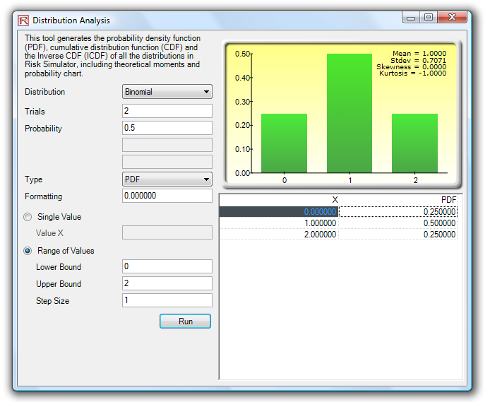 Figure 15.20: Distributional Analysis Tool (Binomial Distribution with 2 Trials)
As a side note, the binomial distribution describes the number of times a particular event occurs in a fixed number of trials, such as the number of heads in 10 flips of a coin or the number of defective items out of 50 items chosen. The three conditions underlying the binomial distribution are:
- For each trial, only two outcomes are possible that are mutually exclusive.
- The trials are independent—what happens in the first trial does not affect the next trial.
- The probability of an event occurring remains the same from trial to trial.
The probability of success (p) and the integer number of total trials (n) are the distributional parameters. The number of successful trials is denoted x. It is important to note that probability of success (p) of 0 or 1 are trivial conditions and do not require any simulations, and, hence, are not allowed in the software.
Input requirements:
Probability of success > 0 and < 1 (that is, 0.0001 ≤ p ≤ 0.9999)
Number of trials ≥ 1 or positive integers and ≤ 1000 (for larger trials, use the normal distribution with the relevant computed binomial mean and standard deviation as the normal distribution’s parameters).
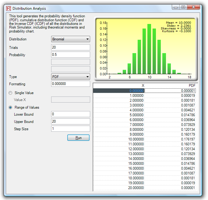
Figure 15.21: Distributional Analysis Tool (Binomial Distribution with 20 Trials)
Figure 15.22 shows the same binomial distribution but now the CDF is computed. The CDF is simply the sum of the PDF values up to the point x. For instance, in Figure 15.21, we see that the probabilities of 0, 1, and 2 are 0.000001, 0.000019, and 0.000181, whose sum is 0.000201, which is the value of the CDF at x = 2 in Figure 15.22. Whereas the PDF computes the probabilities of getting exactly 2 Heads, the CDF computes the probability of getting no more than 2 Heads or up to 2 Heads (or probabilities of 0, 1, and 2 Heads). Taking the complement (i.e., 1 – 0.00021) obtains 0.999799, or 99.9799%, which is the probability of getting at least 3 Heads or more.
As another example, out of 20 projects where there is a 50% independent chance of success of each project, the probability of getting at least 8 successful projects is 86.84% (i.e., the sum of the probabilities of exactly 8, 9, 10, …, 20 successful projects or 100% – the cumulative probability of 0 to 7 from Figure 15.22, or 100% – 13.16% = 86.84%). Alternatively, out of 20 independent projects, the probability of having no more than 12 successful projects is 86.84% (CDF of 12 is 86.84% in Figure 15.22). The probability in this example is the same due to the 50% success probability in a binomial distribution which creates a symmetrical distribution (8 failures is the same as 12 successes out of 20 projects).
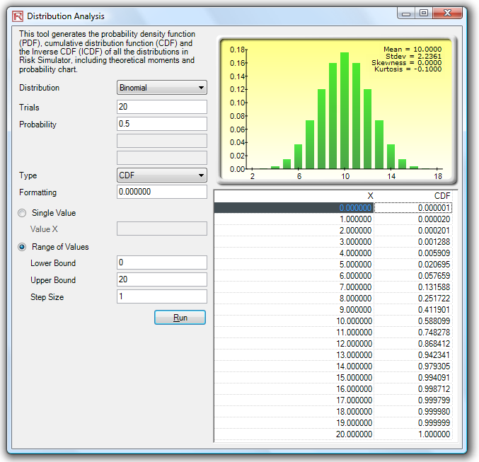
Figure 15.22: Distributional Analysis Tool (Binomial Distribution’s CDF with 20 Trials)
Using this distributional analysis tool, distributions even more advanced can be analyzed, such as the gamma, beta, negative binomial, and many others in Risk Simulator. As further example of the tool’s use in a continuous distribution and the ICDF functionality, Figure 15.23 shows the standard-normal distribution (normal distribution with a mean or mu of zero and standard deviation or sigma of one), where we apply the ICDF to find the value of x that corresponds to the cumulative probability of 97.50% (CDF). That is, a one-tail CDF of 97.50% is equivalent to a two-tail 95% confidence interval (there is a 2.50% probability in the right tail and 2.50% in the left tail, leaving 95% in the center or confidence interval area, which is equivalent to a 97.50% area for one tail). The result is the familiar Z-Score of 1.96. Therefore, using this distributional analysis tool, the standardized scores for other distributions and the exact and cumulative probabilities of other distributions can all be obtained quickly and easily. See the exercises at the end of this chapter for more hands-on applications using the binomial, negative binomial, and other distributions.
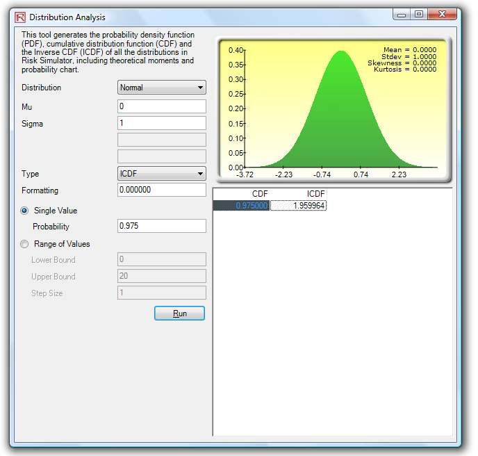
Figure 15.23: Distributional Analysis Tool (Normal Distribution’s ICDF and Z-score)