The Analytical Models modules contain models on estimating and valuing PD, EAD, LGD, Volatility, Credit Exposures, Options-based Asset Valuation, Debt Valuation, Credit Conversion Factors (CCF), Loan Equivalence Factors (LEQ), Options Valuation, Hedging Ratios, and multiple other models. In Basel III/IV/III, the regulations specifically state that all Over-the-Counter (OTC) options, options-embedded instruments, and other exotic options need to also be valued and accounted for. This requirement is why CMOL has devoted an entire module to modeling and valuing these exotic nonlinear instruments. The module is divided into four categories depending on their required inputs and structure of the model. In other words, you might see analytical types like Probability of Default or Volatility traversing multiple tabs or analytical segments.
Figure 1.11 illustrates the Analytical Models tab with input assumptions and results. This analytical model segment is divided into Structural, Time-Series, Portfolio, and Analytics models. The current figure shows the Structural models tab where the computed models pertain to credit risk–related model analysis categories such as PD, EAD, LGD, and Volatility calculations. Under each category, specific models can be selected to run. Selected models are briefly described, and users can select the number of model repetitions to run and the decimal precision levels of the results. The data grid in the Computations tab shows the area in which users would enter the relevant inputs into the selected model and the results would be computed. As usual, selected models, inputs, and settings can be saved for future retrieval and analysis.
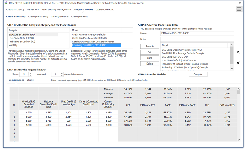
Figure 1.11: Structural Credit Risk Models
Figure 1.11 illustrates the Structural Analytical Models tab with visual chart results. The results computed are displayed as various visual charts such as bar charts, control charts, Pareto charts, and time-series charts. Figure 1.12 illustrates the Time-Series Analytical Models tab with input assumptions and results. The analysis category and model type is first chosen where a short description explains what the selected model does, and users can then select the number of models to replicate as well as decimal precision settings. Input data and assumptions are entered in the data grid provided (additional inputs can also be entered if required), and the results are computed and shown. As usual, selected models, inputs, and settings can be saved for future retrieval and analysis. Figure 1.13 illustrates the Portfolio Analytical Models tab with input assumptions and results. The analysis category and model type are first chosen where a short description explains what the selected model does, and users can then select the number of models to replicate as well as decimal precision settings. Input data and assumptions are entered in the data grid provided (additional inputs such as a correlation matrix can also be entered if required), and the results are computed and shown.
Additional models are available in the Credit Models tab with input assumptions and results. The analysis category and model type are first chosen and input data and assumptions are entered in the required inputs area (if required, users can Load Example inputs and use these as a basis for building their models), and the results are computed and shown. Scenario tables and charts can be created by entering the From, To, and Step Size parameters, where the computed scenarios will be returned as a data grid and visual chart. As usual, selected models, inputs, and settings can be saved for future retrieval and analysis.
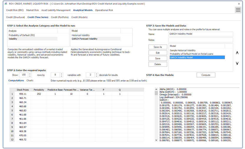
Figure 1.12: Time-Series Credit and Market Models
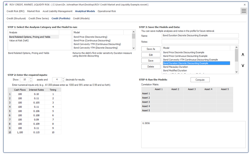
Figure 1.13: Credit Portfolio Models