With all the talk about normality and the need to assume normality in your dataset, below is a list of the most common tests for the normality of a data variable. The most powerful tests are the parametric distributional fitting routines, and the less powerful are the nonparametric and graphical approaches.
- Distributional Fitting. Which distribution does an analyst or engineer use for an input variable in a model? What are the relevant distributional parameters? The null hypothesis tested is that the fitted distribution is the same distribution as the population from which the sample data to be fitted comes.
-
- Akaike Information Criterion (AIC). This method rewards goodness-of-fit but also includes a penalty that is an increasing function of the number of estimated parameters (although AIC penalizes the number of parameters less strongly than other methods).
- Anderson–Darling (AD). When applied to testing if a normal distribution adequately describes a set of data, it is one of the most powerful statistical tools for detecting departures from normality and is powerful for testing normal tails. However, in non-normal distributions, this test lacks power compared to others.
- Kolmogorov–Smirnov (KS). This is a nonparametric test for the equality of continuous probability distributions that can be used to compare a sample with a reference probability distribution, making it useful for testing abnormally-shaped distributions and non-normal distributions.
- Kuiper’s Statistic (K). Related to the KS test, Kuiper’s Statistic is as sensitive in the tails as at the median and is invariant under cyclic transformations of the independent variable. This test is invaluable when testing for cyclic variations over time. In comparison, the AD provides equal sensitivity at the tails as the median, but it does not provide the cyclic invariance.
- Schwarz/Bayes Information Criterion(SC/BIC). The SC/BIC introduces a penalty term for the number of parameters in the model, with a larger penalty than AIC.
- Discrete (Chi-Square). The Chi-Square test is used to perform distributional fitting on discrete data.
- Box–Cox Normal Transformation. Although this is not strictly a test for normality, it takes your existing dataset and transforms it into normally distributed data. The original dataset is tested using the Shapiro–Wilk test for normality (H0: data is assumed to be normal), then transformed using the Box–Cox method either using your custom Lambda parameter or internally optimized Lambda. The transformed data is tested again for normality using Shapiro–Wilk.
- Grubbs Test for Outliers. The Grubbs test is used to identify potential outliers and to test the null hypothesis that all the values are from the same normal population with no outliers.
- Nonparametric Chi-Square Goodness-of-Fit for Normality (Grouped Data). The chi-square test for goodness-of-fit is used to examine if a sample dataset could have been drawn from a population having a specified probability distribution. The probability distribution tested here is the normal distribution. The null hypothesis tested is such that the sample is randomly drawn from the normal distribution.
- Nonparametric Lilliefors Test for Normality. The Lilliefors test evaluates the null hypothesis of whether the data sample was drawn from a normally distributed population, versus an alternate hypothesis that the data sample is not normally distributed. If the calculated p-value is less than or equal to the alpha significance value, then reject the null hypothesis and accept the alternate hypothesis. Otherwise, if the p-value is higher than the alpha significance value, do not reject the null hypothesis. This test relies on two cumulative frequencies: one derived from the sample dataset and one from a theoretical distribution based on the mean and standard deviation of the sample data. An alternative to this test is the chi-square test for normality. The chi-square test requires more data points to run compared to the Lilliefors test.
- Nonparametric: D’Agostino–Pearson Normality Test. The D’Agostino–Pearson test is used to nonparametrically determine if there is near-normality in the dataset. This tests the null hypothesis that the data is normally distributed.
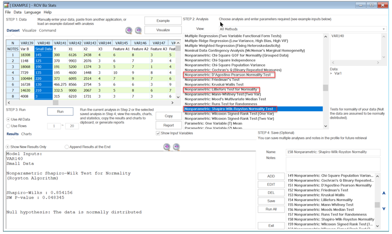
- Nonparametric: Shapiro–Wilk–Royston Normality Test. The Shapiro–Wilk test for normality uses the Royston algorithm to test the null hypothesis that the data is normally distributed.
- Q-Q Normal The Quantile-Quantile chart is a normal probability plot, which is a graphical method for comparing a probability distribution with the normal distribution by plotting their quantiles against each other. It only provides a visual inspection of the near normality of your dataset.
- Skew and Kurtosis: Shapiro–Wilk and D’Agostino–Pearson. You can run the Skew and Kurtosis tests to see if the data has both statistics equal to zero. A normal distribution has skew and kurtosis equal to zero. The D’Agostino–Pearson tests if both skew and kurtosis of the data are simultaneously statistically equal to zero. The null hypothesis is the data has zero skew and zero kurtosis, approximating normality.