File Name: Simulation – DCF, ROI and Volatility
Location: Modeling Toolkit | Risk Simulator | DCF, ROI and Volatility
Brief Description: Illustrates how to use Risk Simulator for running a Monte Carlo simulation in a financial return on investment (ROI) analysis, incorporating various correlations among variables (time-series and cross-sectional relationships), and calculating forward-looking volatility based on the PV Asset approach
Requirements: Modeling Toolkit, Risk Simulator
This is a generic discounted cash flow (DCF) model showing the net present value (NPV), internal rate of return (IRR), and return on investment (ROI) calculations. This model can be adapted to any industry and is used to illustrate how a Monte Carlo simulation can be applied to actual investment decisions and capital budgeting. In addition, the project’s or asset’s volatility is also computed in this example model. Volatility is a measure of risk and is a key input in financial options and real options analysis.
Procedure
To run this model, simply click on Risk Simulator | Run Simulation. However, if you wish you can create your own simulation model:
- Start a new simulationprofile and add various assumptions on the price and quantity inputs.
- Remember to add correlationsbetween the different years of price and quantity (autocorrelation).
- Continue to add correlationsbetween price and quantity (cross-correlations).
- Add forecaststo the key outputs (NPV and Intermediate X Variable to obtain the project’s volatility).
Results Interpretation
If you run the existing simulation profile, you will obtain two forecast charts, the NPV and Intermediate X forecasts.
- From the NPV forecast chart(Figure 140.1), select Two-Tail and enter in 95 in the Certainty box, and hit TAB on the keyboard. The results show that the 95% confidence interval for the NPV falls between $2429 and $3485. If you click on the Statistics tab, the expected value or mean shows the value of $2941. Alternatively, select Left-Tail and enter in 5 in the Certainty box, and hit TAB. The results indicate that the 5% worst-case scenario will still yield a positive NPV of $2488, indicating that this is a good project. You can now compare this with other projects to decide which project should be chosen. Finally, because probabilities of left and right tails in the same forecast distribution are complementary, if you select Right-Tail and enter 2.5 in the Certainty box and hit TAB, the result is $3485, identical to the 95% confidence level’s right-tail value (95% confidence interval means there is a 2.5% probability in each tail).
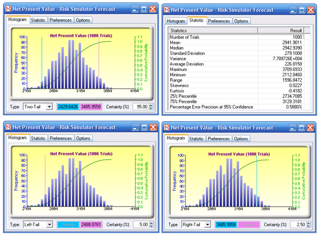
Figure 140.1: NPV forecast results
- The Intermediate X Variable is used to compute the project’s volatility. To obtain a volatility measure, first, modify the model as appropriate and then click on Set Static CF in the model (near cell B46) to generate a static cash flow. Then RUN the simulation and view the Intermediate Variable X’s forecast chart (Figure 140.2). Go to the Statistics tab and obtain the standard deviation, and annualize it by multiplying the value with the square root of the number of periods per year In this case, the annualized volatility is 6.45% as the periodicity of the cash flows in the model is annual, otherwise multiply the standard deviation by the square root of 4 if quarterly data is used, or the square root of 12 if monthly data is used, and so forth.
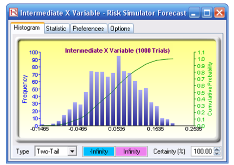
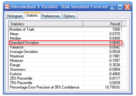
Figure 140.2: Forecast results of the X variable