File Name: Yield Curve – U.S. Treasury Risk-free Rates and Yield Curve – Spline Interpolation and Extrapolation
Location: Modeling Toolkit | Yield Curve | U.S. Treasury Risk-free Rates and Modeling Toolkit | Yield Curve | Spline Interpolation and Extrapolation
Brief Description: Illustrates how to use Risk Simulator for applying distributional fitting and computing volatilities of risk-free rates (application of a Cubic Spline curve to interpolate and extrapolate missing risk-free rates also includes)
Requirements: Modeling Toolkit, Risk Simulator
This model shows the daily historical yield of the U.S. Treasury securities, from 1 month to 30 years, for the years 1990 to 2006. The volatilities of these time-series yields are also computed, and they are then put through a distributional fitting routine in Risk Simulator to determine if they can be fitted to a particular distribution and hence used in a model elsewhere.
There are several ways to compute the volatility of a time series of data, including:
- Logarithmic Cash Flow or Stock Returns Approach: This method is used mainly for computing the volatility on liquid and tradable assets, such as stocks in financial options; however, sometimes it is used for other traded assets, such as the price of oil and electricity. The drawback is that discounted cash flow models with only a few cash flows generally will overstate the volatility, and this method cannot be used when negative cash flows occur. The benefits include its computational ease, transparency, and modeling flexibility of the method. In addition, no simulation is required to obtain a volatility estimate.
- Logarithmic Present Value Returns Approach: This approach is used mainly when computing the volatility on assets with cash flow A typical application is in real options. The drawback of this method is that simulation is required to obtain a single volatility, and it is not applicable for highly traded liquid assets such as stock prices. The benefits include the ability to accommodate certain negative cash flows. Also, this approach applies more rigorous analysis than the logarithmic cash flow returns approach, providing a more accurate and conservative estimate of volatility when assets are analyzed.
- Management Assumptions and Guesses: This approach is used for both financial options and real options. The drawback is that the volatility estimates are very unreliable and are only subjective best guesses. The benefit of this approach is its simplicity––using this method, you can easily explain to management the concept of volatility, both in execution and interpretation.
- Generalized Autoregressive Conditional Heteroskedasticity (GARCH) Models: These methods are used mainly for computing the volatility of liquid and tradable assets, such as stocks in financial options. However, sometimes they are used for other traded assets, such as the price of oil or electricity. The drawback is that these models require a lot of data and advanced econometric modeling expertise is required. In addition, these models are highly susceptible to user manipulation. The benefit is that rigorous statistical analysis is performed to find the best-fitting volatility curve, providing different volatility estimates over time.
This model applies the first method and only describes the approach on a very superficial level. For detailed technical details on volatility estimates, including the theory and step-by-step interpretation of the method, please refer to Chapter 7 of Dr. Johnathan Mun’s Real Options Analysis, Third Edition (Thomson–Shore, 2016).
The Risk-Free Rate Volatility worksheet shows the computed annualized volatilities for each term structure, together with the average, median, minimum, and maximum values. These volatilities are also fitted to continuous distributions and the results are shown in the Fitting Volatility worksheet. Notice that longer-term yields tend to have smaller volatilities than shorter-term more liquid and highly traded instruments.
Procedure
The volatilities and their distributions have already been determined in this model. To review them, follow these instructions:
- Select any of the worksheets(1990 to 2006) and look at the historical risk-free rates as well as how the volatilities are computed using the logarithmic returns approach.
- Go to the Fitting Volatility worksheet and view the resulting fitted distributions, their p-values, theoretical versus empirical values, and cross-correlations (Figure 168.1).
- Notice that in most cases, the p-values are pretty high. For example, the p-value for the 3-month volatilities for the past 17 years is 0.9853, or roughly, about 98.53% of the fluctuations in the actual data can be accounted for by the fitted lognormal distribution, which is indicative of an extremely good fit. We can use this information to model and simulate short-term volatilities very robustly. In addition, the cross-correlations indicate that yields of closely related terms are highly correlated, but the correlation decreases over time. For instance, the 3-month volatilities tend to be highly correlated to the 6-month volatilities but only have negligible correlations to longer-term yields’ (e.g., 10-year) volatilities. This is highly applicable for simulating and modeling options-embedded instruments, such as options-adjusted spreads, which require the term structure of interest rates and volatility structure.
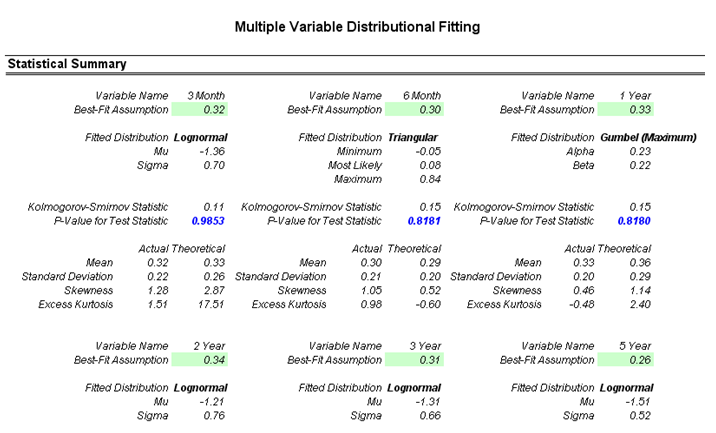
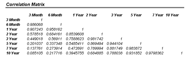
Figure 168.1: P-values and cross-correlations of fitting routines
To replicate the distributional fitting routine, follow the instructions below. You can perform a single-variable fitting and replicate the steps for multiple variables or perform a multiple-fitting routine once. To perform individual fits:
- Start a new profile by clicking on Risk Simulator | New Simulation Profile and give it a name.
- Go to the Risk-Free Rate Volatility worksheet and select a data column (e.g., select cells K6:K22).
- Start the single-fitting procedure by clicking on Risk Simulator | Analytical Tools | Distributional Fitting (Single-Variable).
- Select Fit to Continuous Distributions and make sure all distributions are checked (by default) and click OK.
- Review the results. Note that the best-fitting distribution is listed or ranked first, complete with its p-value. A high p-value is considered statistically to be a good fit. That is, the null hypothesis that the fitted distribution is the right distribution cannot be rejected; therefore, we can conclude that the distribution fitted is the best fit. Thus, the higher the p-value, the better the fit. Alternatively, you can roughly think of the p-value as the percentage fit, for example, the Gumbel Maximum Distribution fits the 10-year volatilities at about 95.77%. You also can review the theoretical and empirical statistics to see how closely the theoretical distribution matches the actual empirical data. If you click OK, a single-fit report will be generated together with the assumption. See Figure 168.2.
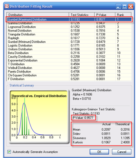
Figure 168.2: Distributional fitting results
Alternatively, you can perform a multiple-variable fitting routine to fit multiple variables at the same time. The problem here is that the data must be complete. In other words, there must be no gaps in the area selected. Looking at the Risk-Free Rate Volatility worksheet, there are gaps as in certain years, the 1-month Treasure Bill, 20-year Treasury Note, and 30-year Treasury Bond are not issued, hence the empty cells. You may have to perform a multi-variable fitting routine on the 3-month to 10-year volatilities and perform single-variable fits on the remaining 1-month, 20-year, and 30-year issues. To perform a multi-variable fit, follow these steps:
- Make sure you have already created a simulationprofile. Then, select the cells D6:K22 and start the multi-fit routine: Risk Simulator | Analytical Tools | Distributional Fitting (Multi-Variable).
- You can rename each of the variables if desired, and make sure that the distributiontypes are all set to Continuous. Click OK when ready. A multiple distribution fitting report will then be generated (see the Fitting Volatility spreadsheet). See Figure 168.3.
Figure 168.3: Multiple fitting result
Cubic Spline Curves
The cubic spline polynomial interpolation and extrapolation model is used to “fill in the gaps” of missing values in a time-series dataset. In this chapter, we illustrate the model application on spot yields and the term structure of interest rates whereby the model can be used to both interpolate missing data points within a time series of interest rates (as well as other macroeconomic variables such as inflation rates and commodity prices or market returns) and also used to extrapolate outside of the given or known range, useful for forecasting purposes.
To illustrate, Figure 168.4 shows the published zero-coupon government bonds (risk-free rates) issued by the U.S. Department of Treasury. The values provided are 1-month, 3-month, 6-month, 1–3 years, and then skips to years 5, 7, 10, 20, and 30. We can apply the cubic spline methodology to interpolate the missing values from 1 month to 30 years, and extrapolate beyond 30 years. Figure 168.5 shows the interest rates plotted as a yield curve, and Figure 168.6 shows how to run the cubic spline forecasts. You can use either Modeling Toolkit’s MTCubicSpline function or Risk Simulator | Forecasting | Cubic Spline. The Known X Values input are the values on the x-axis (in the example, we are interpolating interest rates, a time series of values, making the x-axis time). The Known Y Values are the published interest rates. With this information, we can determine the required Y values (missing interest rates) by providing the required X values (the time periods where we want to predict the interest rates).
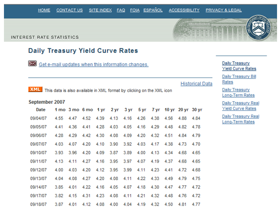
Figure 168.4: Sample U.S. Treasury risk-free interest rates
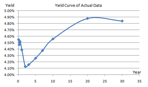
Figure 168.5: Yield curve of published rates
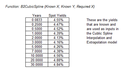
Figure 168.6: Modeling cubic spline
Figure 168.7 shows the results from a cubic spline forecast. The entire term structure of interest rates for every six months is obtained, from the period of 6 months to 50 years. The interest rates obtained up to year 30 are interpolated. Interest rates beyond year 30 are extrapolated from the original known dataset. Notice that the time-series chart shows a nonlinear polynomial function that is obtained using spline curve methodology.
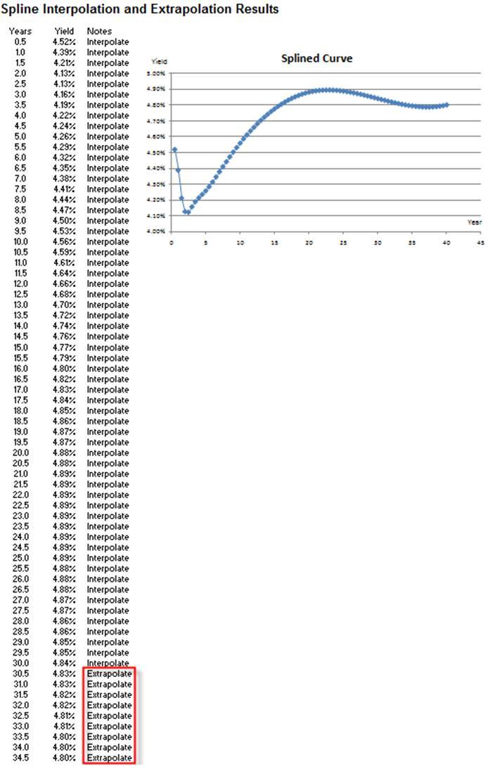
Figure 168.7: Cubic spline results