Figures 7.1–7.4 illustrate the use of PEAT’s S-Curve Costing Model to run the WBS cost simulation for cost, risks, and opportunities. The following provides some additional information on how the model is set up and run in the software:
- Input Assumptions. This is where the Cost, Risk, Opportunity, and Risk Spreads are entered for the program.
- Risk Simulation. This is the heart of the tool where the risk simulationis performed and the resulting S-Curves are obtained, including all the ancillary statistics.
- Return on Sales. This module computes the various government bid contract types, such as Cost Plus Award Fee, Cost Plus Incentive Fee, Cost Plus Fixed Fee, Firm Fixed Price, Fixed Price Incentive Firm, and Fixed Price Incentive Successive Targets, and utilizes the results of risk simulated percentiles in its computations.
- Range of Financial Outcomes. This module takes the results from the Return on Sales (ROS) tab and provides a summary of the range of financial outcomes and returns the most critical pieces of information from the ROS model.
- Knowledge Center. This module includes a quick set of S-Curve Lessons (the basics of interpreting S-Curves), Getting Started Videos (quick lessons and introductions on using the tool), and Step by Step Procedures (this includes quick getting started steps in using the tool, that provide the analyst with a jump start instead of having to read lengthy user manuals).
In the software, click on File | Load Example to run a default example model with preconfigured settings and data (Figure 7.1). By default, the first tab shown is the Input Assumptions tab, showing the Cost, Risk, Opportunity, and Spread Tables subtabs with previously entered and saved data.
In the Cost subtab, some data already exists for you to get started. You can, in your own model, manually type in the data or copy and paste your data into the grid. Simply copy your data from another source (such as a text file, Word document, Excel file, etc.), select the cell or cells you wish to paste, and click on Edit | Paste or right-click and select Paste. Enter or paste your cost WBS Items and the Expected Value, and select the Risk Spread as appropriate for each WBS row.
Repeat the same steps above in the Risk and Opportunity subtabs. However, in those tabs, there is an extra column called Probability that requires input.
The data input portion of this tool is relatively straightforward but the following are some helpful tips to increase your productivity in using the tool:
- Columns that are inputs are colored white, whereas computed cells/columns are a light gray color. Also, not being able to click on a cell and type in a value indicates that that cell or column is a calculated output (e.g., Computed Low/High columns).
- Selecting the Spread from the drop-down list will automatically compute the Computed High/Low columns based on the spread level and distribution type selected. The Spreads are based on the Spread Tables subtab, which we will explore in a moment.
- The Expected Value column is user input and comprises static input values, whereas the Simulation column would be the computed/simulated results. When we run a risk simulation in the next few steps, you will see the values in this column dynamically change.
- The default is to show 100 rows, but you can change the number of rows to view as required. The same goes for the number of decimals to show (default is 0 decimals, where values are rounded to the nearest dollar). Please make sure you have enough rows before pasting data, otherwise, there might be some missing data rows, or after pasting data, do not reduce the number of rows to less than the rows of data you have (of course, you will get a warning message if this happens) as some data might be accidentally deleted.
- You can also Reset All Spreads at once using the drop-down list on the top right of the user interface. This will reset all the Spreads for the subtab.
- File | Data Encryption and Decryption allows you to protect your data.
- Pasting data will only work on the white input cells. You cannot paste data on computed cells or a droplist like Risk Spreads.
- Edit | Edit Spreads Droplist allows you to configure which risk spreads are available in which of the Cost, Risk, or Opportunity subtabs.
- The headers can be clicked to sort the data. However, to facilitate sorting the dataset without empty rows, the tool will automatically reduce the number of visible rows to match the number of available rows of data before performing the sort. By sorting, you can look at WBS line items grouped by risk spreads or arranged in terms of expected value, and so forth.
- The Spread droplist can be copy and pasted. That is, you can select a spread for a specific line item, right-click Copy and then select multiple other rows and right-click Paste the same risk spread. This comes in handy when the WBS structure is large.
In the Spread Tables subtab (Figure 7.4) in the Input Assumptions tab is where the default risk spreads are entered. Continuing with the same example, click on the Spread Tables subtab in the main Input Assumptions tab.
The Triangular subtab shows the default Symmetrical, Left Skew, and Right Skew distributions for a Triangular distribution and the 7 risk levels of each distribution skew-type. You can override these Low and High risk spread values but remember to click on File | Save to retain the changes or click on the Restore Default Spreads button to restore the default values if you make a mistake.
The following are some important notes to keep in mind when it comes to the risk spread tables:
- The Normal subtab shows the normal distribution’s risk spread levels, just like the Triangular subtab, where you can change the spreads as required or keep the default values.
- In contrast, the Program Specific, or Custom, subtab allows you to enter your own Risk Level Names and Risk Level Spreads specific for the program under evaluation, up to 20 risk levels.
- When you edit or enter Custom Spreads, it Auto-Saves without prompting. When you re-open the software tool the next time, the entered custom spreads will be present.
- You can edit/change the default spreads by going to the installation path folder and editing the Default Spreads.xml file directly. You can edit this file in Notepad or Word, but please take care when doing so, as the current default spreads are based on the Air Force Cost Analysis Manual guidelines. The spreads in the tool cannot be edited directly to prevent any user errors.
- There is a New Subcategory available under the customized categories. This New Subcategory just creates an empty row devoid of any numerical inputs; whatever you put on this line is not used or calculated, but only used as a visual separation, such as if the user wants to say the following section is Level 3 rollup or Level 2 rollup of the WBS or a separate group of data/category within a WBS. This is not available by default but can be turned on easily. Simply go to Edit | Edit Spread List and check the New Subcategory selection at the bottom.
- If No Selection is made for a risk spread (i.e., either by not selecting something or selecting the blank line) this line item is taken out of the computation mix completely. In other words, no selection is like a placeholder for the user to temporarily put a line item in, but the inputs are not used in the calculations… this provides the user with some flexibility! Compare this to the drop-list selection of No Risk which means this line item is not simulated but the single-point expected value input is still used in the calculations.
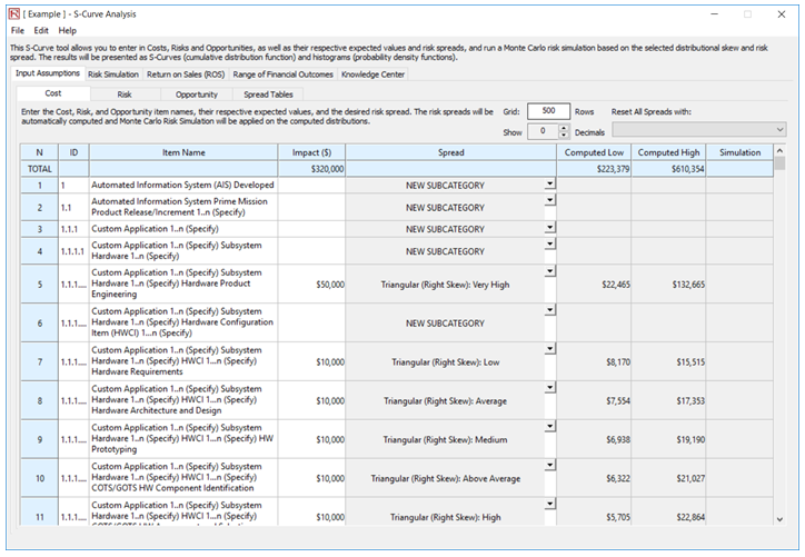
Figure 7.1: S-Curve Cost Pricing Software’s Work Breakout Structure Costs
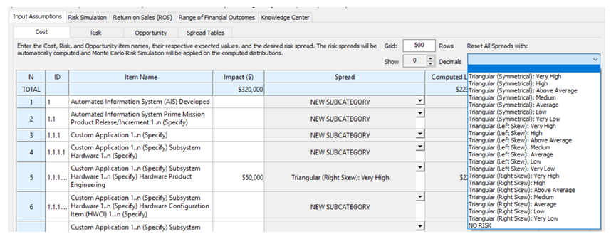
Figure 7.2: Simulation Assumption Spreads
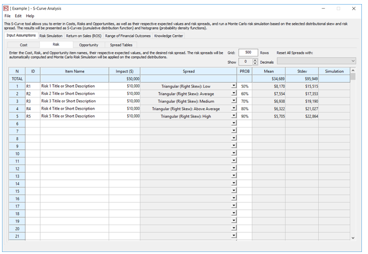
Figure 7.3: Risks
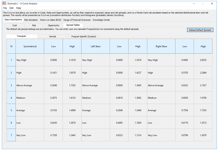
Figure 7.4: Simulation Spread Tables
Results Interpretation
Figure 7.5 shows the results from a Monte Carlo risk simulation. The CDF or cumulative distribution function is shown as a typical S-curve shape. Depending on the decision maker, the typical level to use in a bid is 75th to 85th percentile. In the current example, the 80th percentile is a bid price of $433,665. This result would not be possible and cannot be obtained without running a simulation. For example, single-point estimates would yield a total of $223,379 when summing all the minimum values and $610,354 if all maximum values are added together in the WBS.
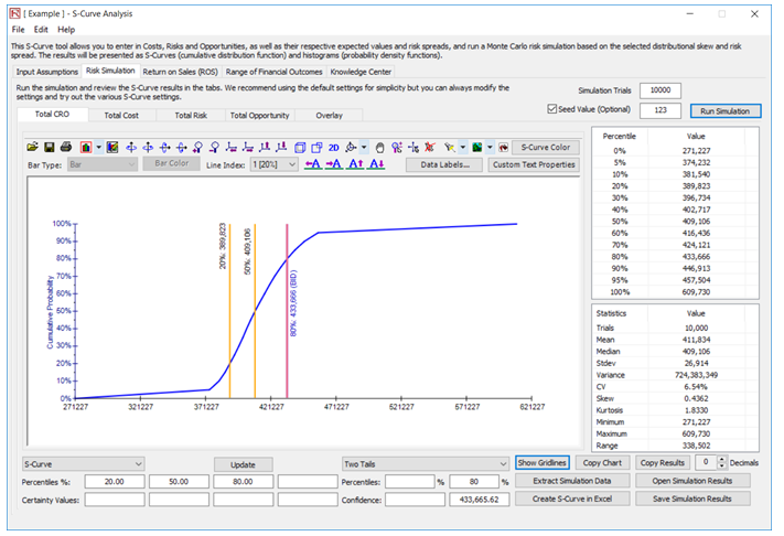
Figure 7.5: Simulated Cost Pricing S-Curve
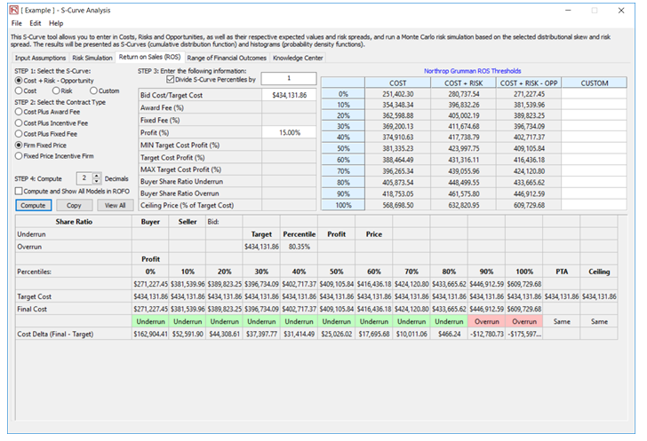
Figure 7.6: CRO Analysis Based on Contract Types