File Names: Real Options – Expansion American and European Option; Real Options – Expansion Bermudan Option; Real Options – Expansion Customized Option
Location: Modeling Toolkit | Real Options Models
Brief Description: Computes expansion options with multiple flavors (American, Bermudan, and European) with customizable and changing inputs using closed-form and customized binomial lattices
Requirements: Modeling Toolkit, Real Options SLS
The Expansion Option values the flexibility to expand from a current existing state to a larger or expanded state. Therefore, an existing state or condition must be present in order to use the expansion option. That is, there must be a base case on which to expand. If there is no base case state, then the simple Execution Option (calculated using the simple Call Option) is more appropriate, where the issue at hand is whether to execute a project immediately or to defer execution.
As an example, suppose a growth firm has a static valuation of future profitability using a DCF model (in other words, the present value of the expected future cash flows discounted at an appropriate market risk-adjusted discount rate) that is found to be $400 million (PV Asset). Using Monte Carlo simulation, you calculate the implied Volatility of the logarithmic returns on the assets based on the projected future cash flows to be 35%. The Risk-Free Rate on a riskless asset (five-year U.S. Treasury note with zero coupons) for the next five years is found to be 7%.
Further, suppose that the firm has the option to expand and double its operations by acquiring its competitor for a sum of $250 million (Implementation Cost) at any time over the next five years (Maturity). What is the total value of this firm, assuming that you account for this expansion option? The results in Figure 182.1 indicate that the strategic project value is $638.73M (using a 10-step lattice), which means that the expansion option value is $88.73M. This result is obtained because the NPV of executing immediately is $400M × 2 – $250M, or $550M. Thus, $638.73 less $550M is $88.73M, the value of the ability to defer and to wait and see before executing the expansion option. The example file used is Expansion American and European Option.
Increase the dividend rate to, say, 2% and notice that both the American and European Expansion Options are now worth less, and that the American Expansion Option is worth more than the European Expansion Option by virtue of the American Option’s ability to be executed early (Figure 182.2). The dividend rate is the cost of waiting to expand or to defer and not execute. That is, this rate is the opportunity cost of waiting on executing the option, and the cost of holding the option. If the dividend rate is high, then the ability to defer reduces and the option to wait decreases.
Increase the Dividend Rate to 4.9% and see that the binomial lattice’s Custom Option result reverts to $550, (the static, expand-now scenario), indicating that the option is worthless (Figure 182.3). This result means if the cost of waiting as a proportion of the asset value (as measured by the dividend rate) is too high, then execute now and stop wasting time deferring the expansion decision! Of course, this decision can be reversed if the volatility is significant enough to compensate for the cost of waiting. That is, it might be worth something to wait and see if the uncertainty is too high even if the cost to wait is high.
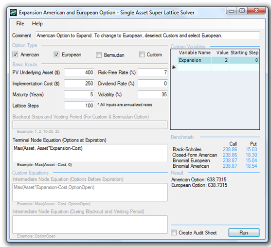
Figure 182.1: American and European options to expand with a 100-step lattice
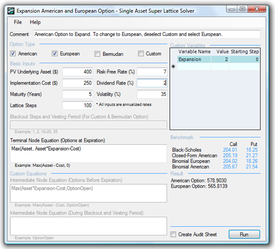
Figure 182.2: American and European options to expand with a dividend rate
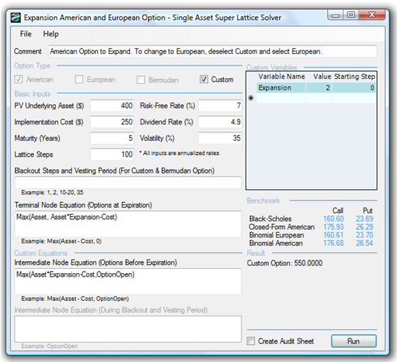
Figure 182.3: Dividend rate optimal trigger value
Other applications of this option abound! To illustrate, here are some additional examples of the contraction option:
- Suppose a pharmaceutical firm is thinking of developing a new type of insulin that can be inhaled and the drug will be absorbed directly into the bloodstream. A novel and honorable idea. Imagine what this means to diabetics, who will no longer need painful and frequent injections. The problem is, this new type of insulin requires a brand-new development If the uncertainties of the market, competition, drug development, and Food and Drug Administration approval are high, perhaps a base insulin drug that can be ingested is developed first. The ingestible version is a required precursor to the inhaled version. The pharmaceutical firm can decide either to take the risk and fast-track development into the inhaled version or to buy an option to defer, to first wait and see if the ingestible version works. If this precursor works, then the firm has the option to expand into the inhaled version. How much should the firm be willing to spend on performing additional tests on the precursor, and under what circumstances should the inhaled version be implemented directly? Suppose the intermediate precursor development work yields an NPV of $100M, but at any time within the next two years, an additional $50M can be invested into the precursor to develop it into the inhaled version, which will triple the NPV. However, after modeling the risk of technical success and uncertainties in the market (competitive threats, sales, and pricing structure), the annualized volatility of the cash flows using the logarithmic present value returns approach comes to 45%. Suppose the risk-free rate is 5% for the two-year period. Using the SLS, the analysis results yields $254.95M, indicating that the option value to wait and defer is worth more than $4.95M after accounting for the $250M NPV if executing now. In playing with several scenarios, the break-even point is found when dividend yield is 1.34%. This means that if the cost of waiting (lost net revenues in sales by pursuing the smaller market rather than the larger market, and loss of market share by delaying) exceeds $1.34M per year, it is not optimal to wait, and the pharmaceutical firm should invest in the inhaled version immediately. The loss in returns generated each year does not sufficiently cover the risks incurred.
- An oil and gas company is currently deciding on a deep-sea exploration and drilling project. The platform provides an expected NPV of $1,000M. This project is fraught with risks (price of oil and production rate are both uncertain) and the annualized volatility is computed to be 55%. The firm is thinking of purchasing an expansion option by spending an additional $10M to build a slightly larger platform that it does not currently need. If the price of oil is high, or when the production rate is low, the firm can execute this expansion option and execute additional drilling to obtain more oil to sell at the higher price, which will cost another $50M, thereby increasing the NPV by 20%. The economic life of this platform is 10 years and the risk-free rate for the corresponding term is 5%. Is obtaining this slightly larger platform worth it? Using the SLS, the option value is worth $27.12M when applying a 100-step lattice. Therefore, the option cost of $10M is worth it. However, this expansion option will not be worth it if annual dividends exceed 0.75% or $7.5M a year—this is the annual net revenues lost by waiting and not drilling as a percentage of the base case NPV.
Figure 182.4 shows a Bermudan Expansion Option with certain vesting and blackout steps, while Figure 182.5 shows a Customized Expansion Option to account for the expansion factor changing over time. Of course, other flavors of customizing the expansion option exist, including changing the implementation cost to expand, and so forth.
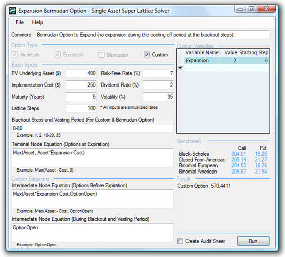
Figure 182.4: Bermudan expansion option
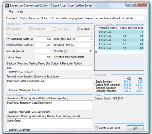
Figure 182.5: Customized expansion option
Exercise: Option to Expand
As another example, suppose a growth firm exists, and its static valuation of future profitability using a DCF model (in other words, the present value of the expected future cash flows discounted at an appropriate market risk-adjusted discount rate) is found to be $400 million. Using Monte Carlo simulation, you calculate the implied volatility of the logarithmic returns on the projected future cash flows to be 35%. The risk-free rate on a riskless asset for the next five years is found to be yielding 7%. Suppose that the firm has the option to expand and double its operations by acquiring its competitor for a sum of $250 million at any time over the next five years. What is the total value of this firm assuming you account for this expansion option?
You decide to use a closed-form approximation of an American call option as a benchmark because the option to expand the firm’s operations can be exercised at any time up to the expiration date. You also decide to confirm the value of the closed-form analysis with a binomial lattice calculation. Do the following exercises, answering the questions that are posed:
- Solve the expansion option problem manually using a 10-step lattice and confirm the results by generating an audit sheet using the software.
- Rerun the expansion option problem using the software for 100 steps, 300 steps, and 1,000 steps. What are your observations?
- Show how you would use the Closed-Form American Approximation Model to estimate and benchmark the results from an expansion option. How comparable are the results?
- Show the different levels of expansion factors but still yielding the same expanded asset value of $800. Explain your observations of why, when the expansion value changes, the Black-Scholes and Closed-Form American Approximation models are insufficient to capture the fluctuation in value.
- Use an expansion factor of 2.00 and an asset value of $400.00 (yielding an expanded asset value of $800).
- Use an expansion factor of 1.25 and an asset value of $640.00 (yielding an expanded asset value of $800).
- Use an expansion factor of 1.50 and an asset value of $533.34 (yielding an expanded asset value of $800).
- Use an expansion factor of 1.75 and an asset value of $457.14 (yielding an expanded asset value of $800).
-
Add a dividend yield and see what happens. Explain your findings.
- What happens when the dividend yield equals or exceeds the risk-free rate?
- What happens to the accuracy of closed-form solutions such as the Black-Scholes and Closed-Form American Approximation models when used as benchmarks?
- What happens to the decision to expand if a dividend yield exists? Now suppose that although the firm has an annualized volatility of 35%, the competitor has a volatility of 45%. This means that the expansion factor of this option changes over time, comparable to the volatilities. In addition, suppose the implementation cost is a constant 120% of the existing firm’s asset value at any point in time. Show how this problem can be solved using the Multiple Asset SLS. Is there option value in such a situation?