Theory
Bootstrap simulation is a simple technique that estimates the reliability or accuracy of forecast statistics or other sample raw data. Bootstrap simulation can be used to answer a lot of confidence- and precision-based questions in simulation. For instance, suppose an identical model (with identical assumptions and forecasts but without any random seeds) is run by 100 different people, the results will clearly be slightly different. The question is, if we collected all the statistics from these 100 people, how will the mean be distributed, or the median, or the skewness, or excess kurtosis? Suppose one person has a mean value of say, 1.50 while another 1.52. Are these two values statistically significantly different from one another or are they statistically similar and the slight difference is due entirely to random chance? What about 1.53? So, how far is far enough to say that the values are statistically different? In addition, if a model’s resulting skewness is –0.19 is this forecast distribution negatively skewed or is it statistically close enough to zero to state that this distribution is symmetrical and not skewed? Thus, if we bootstrapped this forecast 100 times, i.e., run a 1,000-trial simulation for 100 times and collect the 100 skewness coefficients, the skewness distribution would indicate how far zero is away from –0.19. If the 90% confidence on the bootstrapped skewness distribution contains the value zero, then we can state that on a 90% confidence level, this distribution is symmetrical and not skewed, and the value –0.19 is statistically close enough to zero. Otherwise, if zero falls outside of this 90% confidence area, then this distribution is negatively skewed. The same analysis can be applied to excess kurtosis and other statistics.
Essentially, bootstrap simulation is a hypothesis testing tool. Classical methods used in the past relied on mathematical formulas to describe the accuracy of sample statistics. These methods assume that the distribution of a sample statistic approaches a normal distribution, making the calculation of the statistic’s standard error or confidence interval relatively easy. However, when a statistic’s sampling distribution is not normally distributed or easily found, these classical methods are difficult to use. In contrast, bootstrapping analyzes sample statistics empirically by repeatedly sampling the data and creating distributions of the different statistics from each sampling. The classical methods of hypothesis testing are available in Risk Simulator and are explained in the next section. Classical methods provide higher power in their tests but rely on normality assumptions and can only be used to test the mean and variance of a distribution, as compared to bootstrap simulation, which provides lower power but is nonparametric and distribution-free, and can be used to test any distributional statistic.
Procedure
- Run simulation with assumptions and forecasts (e.g., use the Risk Simulator | Example Models | 08 Hypothesis Testing and Bootstrap Simulation).
- Select Risk Simulator | Analytical Tools | Nonparametric Bootstrap.
- Select only one forecast to bootstrap, select the statistic(s) to bootstrap, and enter the number of bootstrap trials and click OK (Figure 15.16).
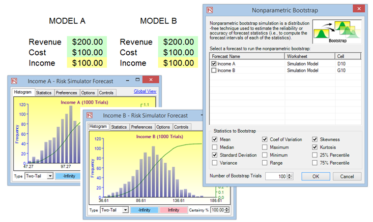
Figure 15.16: Nonparametric Bootstrap Simulation
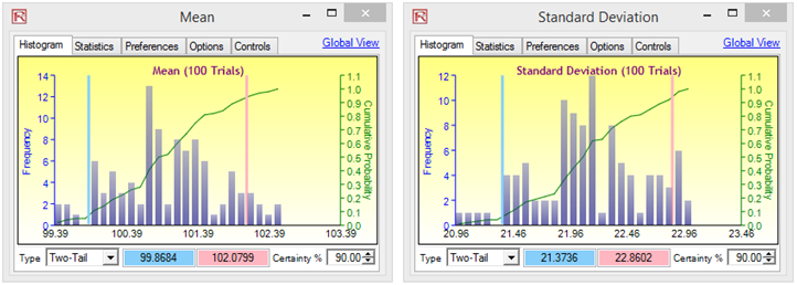
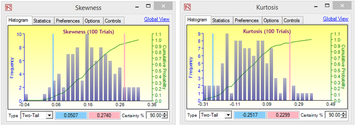
Figure 15.17: Bootstrap Simulation Results
Results Interpretation
Figure 15.17 illustrates some sample bootstrap results. The example file used was Hypothesis Testing and Bootstrap Simulation. For instance, the 90% confidence for the kurtosis statistic is between –0.2517 and 0.2299, such that the value 0 falls within this confidence, indicating that on a 90% confidence, the kurtosis of this forecast is not statistically significantly different from zero, or that this distribution can be considered as normal-tailed. Conversely, if the value 0 falls outside of this confidence, then the opposite is true, the distribution has excess kurtosis skewed (positive kurtosis if indicating fat tails if the forecast statistic is positive, and negative kurtosis with flat-tailed if the forecast statistic is negative). Similarly, in Figure 15.17, we can state that the distribution is positively skewed (the 90% confidence interval is from 0.0507 to 0.2740, and 0 falls outside of this interval).
Notes
The term bootstrap comes from the saying, “to pull oneself up by one’s own bootstraps,” and is applicable because this method uses the distribution of statistics themselves to analyze the statistics’ accuracy. Nonparametric simulation is simply randomly picking golf balls from a large basket with replacement where each golf ball is based on a historical data point. Suppose there are 365 golf balls in the basket (representing 365 historical data points). Imagine if you will that the value of each golf ball picked at random is written on a large whiteboard. The results of the 365 balls picked with replacement are written in the first column of the board with 365 rows of numbers. Relevant statistics (e.g., mean, median, mode, standard deviation, and so forth) are calculated on these 365 rows. The process is then repeated, say, five thousand times. The whiteboard will now be filled with 365 rows and 5,000 columns. Hence, 5,000 sets of statistics (that is, there will be 5,000 means, 5,000 medians, 5,000 modes, 5,000 standard deviations, and so forth) are tabulated and their distributions are shown. The relevant statistics of the statistics are then tabulated, where from these results one can ascertain how confident the simulated statistics are. Finally, bootstrap results are important because according to the Law of Large Numbers and Central Limit Theorem in statistics, the mean of the sample means is an unbiased estimator and approaches the true population mean when the sample size increases.