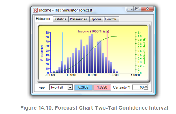
In forecast charts, you can determine the probability of occurrence called confidence intervals. That is, given two values, what are the chances that the outcome will fall between these two values? Figure 14.10 illustrates that there is a 90% probability that the final outcome (in this case, the level of income) will be between $0.2653 and $1.3230. The two-tailed confidence interval can be obtained by first selecting Two-Tail as the type, entering the desired certainty value (e.g., 90), and hitting TAB on the keyboard. The two computed values corresponding to the certainty value will then be displayed. In this example, there is a 5% probability that income will be below $0.2653 and another 5% probability that income will be above $1.3230. That is, the two-tailed confidence interval is a symmetrical interval centered on the median or 50th percentile value. Thus, both tails will have the same probability.
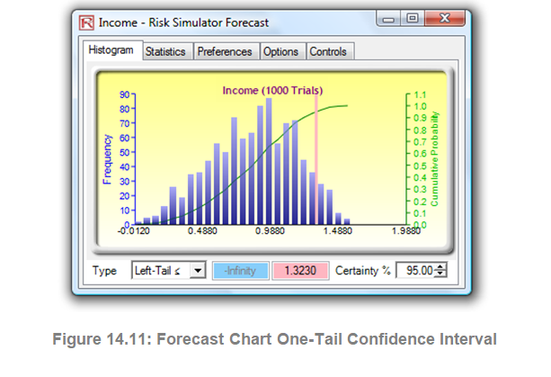
Alternatively, a one-tail probability can be computed. Figure 14.11 shows a Left-Tail selection at 95% confidence (i.e., choose Left-Tail ≤ as the type, enter 95 as the certainty level, and hit TAB on the keyboard). This means that there is a 95% probability that the income will be at or below $1.3230 or a 5% probability that income will be above $1.3230, corresponding perfectly with the results seen in Figure 14.10.
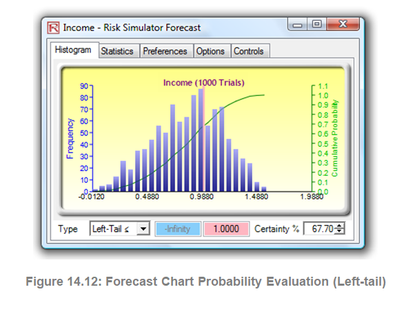
 In addition to evaluating what the confidence interval is (i.e., given a probability level and finding the relevant income values), you can determine the probability of a given income value (Figure 14.12). For instance, what is the probability that income will be less than or equal to $1? To do this, select the Left-Tail ≤ probability type, enter 1 into the value input box, and hit TAB. The corresponding certainty will then be computed (in this case, there is a 67.70% probability income will be at or below $1).
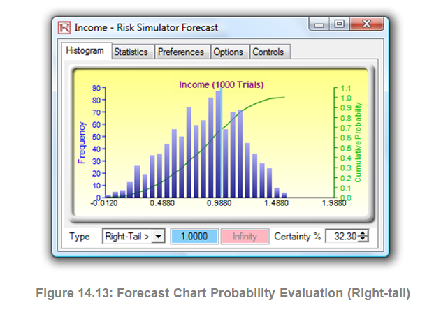
For the sake of completeness, you can select the Right-Tail > probability type and enter the value 1 in the value input box, and hit TAB (Figure 14.13). The resulting probability indicates the right-tail probability past the value 1, that is, the probability of income exceeding $1 (in this case, we see that there is a 32.30% probability of income exceeding $1). The sum of 32.30% and 67.70% is, of course, 100%, the total probability under the curve.
Additional Tips
- The forecast window is resizable by clicking on and dragging the bottom right corner of the forecast window. It is always advisable that before rerunning a simulation, the current simulation should be reset (Risk Simulator | Reset Simulation).
- Remember that you will need to hit TAB on the keyboard to update the chart and results when you type in the certainty values or right- and left-tail values.
- You can also hit the Spacebar on the keyboard repeatedly to cycle among the histogram, statistics, preferences, options, and control tabs.
- In addition, if you click on Risk Simulator | Options, you can access several different options for Risk Simulator, including allowing Risk Simulator to start each time Excel starts or to only start when you want it to (by double-clicking on the Risk Simulator icon on the desktop), change the cell colors of assumptions and forecasts, as well as turn cell comments on and off (cell comments will allow you to see which cells are input assumptions and which are output forecasts as well as their respective input parameters and names). Do spend some time experimenting with the forecast chart outputs and various bells and whistles, especially the Controls tab.
- You can also click on the Global View (top right corner of the forecast charts) to view all the tabs in a single comprehensive interface and return to the regular view by clicking on the Normal View link.