File Name: Simulation – Recruitment Budget (Negative Binomial and Multidimensional Simulation)
Location: Modeling Toolkit | Risk Simulator | Recruitment Budget (Negative Binomial and Multidimensional Simulation)
Brief Description: Illustrates how to use Risk Simulator in applying the Negative Binomial distribution to compute the required budget to obtain the desired outcomes given probabilities of failure, using the Distribution Analysis tool to determine the theoretical probabilities of success, and applying a Multidimensional Simulation approach where the inputs into a simulation are uncertain
Requirements: Modeling Toolkit, Risk Simulator
Negative Binomial Simulation
The negative binomial distribution is useful for modeling the distribution of the number of additional trials required on top of the number of successful occurrences required (R). For instance, in order to close a total of 10 sales opportunities, how many extra sales calls would you need to make above 10 calls given some probability of success in each call? The x-axis shows the number of additional calls required or the number of failed calls. The number of trials is not fixed, the trials continue until the Rth success, and the probability of success is the same from trial to trial. The probability of success (P) and the number of successes required (R) are the distributional parameters. Such a model can be applied in a multitude of situations, such as the cost of cold sales calls, the budget required to train military recruits, and so forth.
The simple example shown illustrates how a negative binomial distribution works. Suppose that a salesperson is tasked with making cold calls and a resulting sale is considered a success while no sale means a failure. Suppose that historically the proportion of sales to all calls is 30%. We can model this using the negative binomial distribution by setting the Successes Required (R) to equal 2 and the Probability of Success (P) as 0.3.
For instance, as illustrated in Figure 142.1, say the salesperson makes two calls. The success rate is 30% per call, and the success or failure of one call versus another are statistically independent of one another. There can be four possible outcomes (SS, SF, FS, FF, where S stands for success, and F for failure). The probability of SS is 0.3 ×0.3 or 9%; SF and FS is 0.3 × 0.7 or 21% each; and FF is 0.7 × 0.7 or 49%. The total probability is 100%. Therefore, there is a 9% chance that two calls are sufficient and no additional calls are required to get the two successes required. In other words, X = 0 has a probability of 9% if we define X as the additional calls required beyond the two calls.
Extending this to three calls, we have many possible outcomes, but the key outcomes we care about are two successful calls, which we can define as the following combinations: SSS, SSF, SFS, and FSS, and their respective probabilities are computed (e.g., FSS is computed by 0.7 × 0.3 × 0.3 = 6.30%). Now, the combinatorial sequence SSS and SSF do not require a third call because the first two calls have already been successful. Further, SFF, FSF, FFS, and FFF all fail the required two-call success as they only have either zero or one successful call. So, the sum total probability of the situations requiring the third call to make exactly two calls successful out of three is 12.60%.
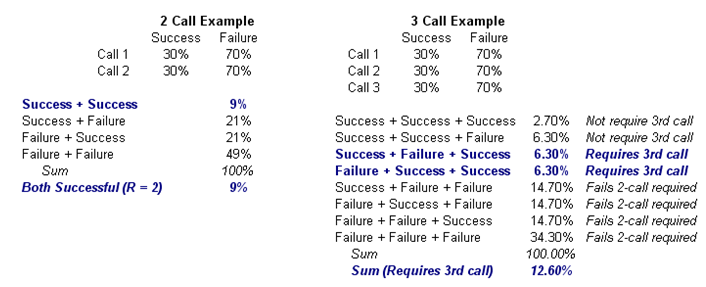
Figure 142.1: Sample negative binomial distribution
Clearly, doing this exercise for a large combinatorial problem with many required successes is difficult and intractable. However, we can obtain the same results using Risk Simulator. For instance, creating a new profile and setting an input assumption, and choosing the negative binomial distribution with R = 2 and P = 0.3 provides the chart in Figure 142.2. Notice that the probability of X = 0 is exactly what we had computed, 9%, and X = 1 yields 12.60%.
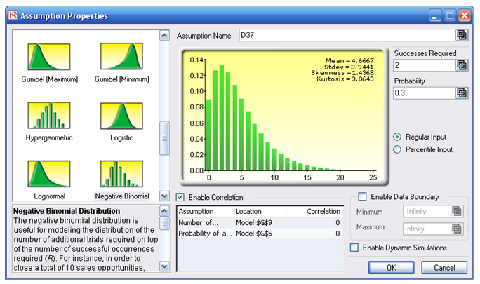
Figure 142.2: Negative binomial distribution
It is easier if you use Risk Simulator’s Distribution Analysis tool (Figure 142.3) to obtain the same results with a table of numerical values. If you choose the PDF type, you obtain the exact probabilities. That is, there is a 12.6% probability you will need to make three calls (or one additional call on top of the required two calls), or 13.23% with four calls, and so forth.
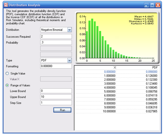
Figure 142.3: Negative binomial distribution’s theoretical PDF properties
If you select CDF (Figure 142.4), the cumulative probabilities will be computed. For instance, the CDF value when X = 1 is 9% + 12.6% or 21.6%, which means that 21.6% of the time, making three calls (or X = 1 extra call beyond the required two) is sufficient to get two successful calls to be, say, 80% sure, you should be prepared to make up to seven additional calls, or nine calls total, but you can stop once two successes have been achieved.
Procedure for Computing Probabilities in a Negative Binomial Distribution
- Start the Distribution Analysis tool (click on Risk Simulator| Tools | Distribution Analysis).
- Select Negative Binomial from the Distribution drop list, and enter 2 for successes required and 3 for the probability of success, then select Range of Values and enter 0 and 10 for the Lower and Upper Bounds, with 1 as the Step Size and click RUN.
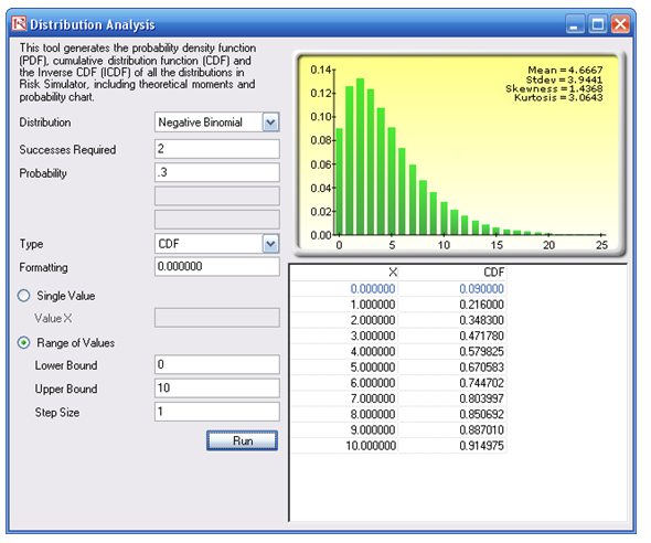
Figure 142.4: Negative binomial distribution’s theoretical CDF properties
Multidimensional Simulation
The Model worksheet shows a simple recruitment budget example, where the task is to determine the total cost required to obtain the required number of qualified and trained recruits, when, in fact, only a small percentage of recruits will successfully complete the training course. The required weeks of training and cost per week are also used as inputs. The question is, how much money (budget) is required to train these recruits given these uncertainties? In Figure 142.5, G9 is a Risk Simulator assumption with a Negative Binomial distribution with R = 10 (linked to cell G4) and P = 0.25 (linked to cell G5). Cell G12 is the model’s forecast. You can now run a simulation and obtain the distribution forecast of the required budget.
In contrast, if the 25% rate is an unknown and uncertain input, you can set it as an assumption, and make the value in cell G9 a link to the 25% cell, and check the box Enable Dynamic Simulation. This means that the value of 25% is an assumption and changes with each trial, and the number of recruits failing is also an assumption but is linked to this changing 25% value. This is termed a multidimensional simulation model (Figure 142.6).
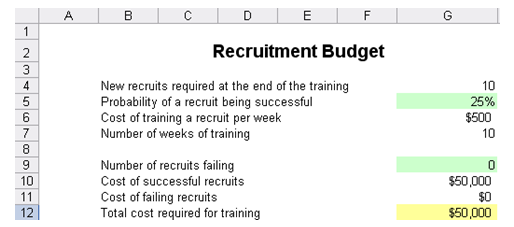
Figure 142.5: Recruitment model
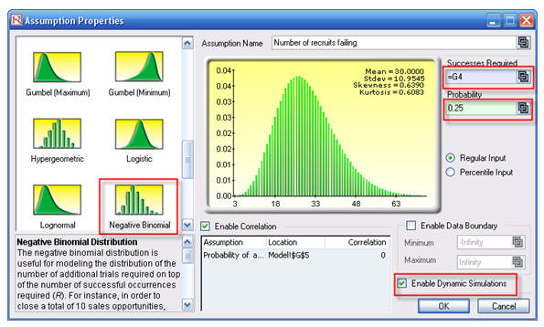
Figure 142.6: Multidimensional simulation assumptions
The results show that on a 90% confidence, the required budget should be between $115,000 and $315,000 (Figure 142.7), with an expected value of $200,875 (Figure 142.8).
Procedure for Running a Multidimensional Simulation
The model is also preset with assumptions and forecasts. To run this model:
- Go to the Model worksheet and click on Risk Simulator | Change Profile and select the Recruitment Budget profile.
- Click on the RUN icon or Risk Simulator | Run Simulation.
- On the forecast chart, select Two-Tail, enter in 90 in the Certainty box, and hit TAB on the keyboard.
To recreate the assumptions and forecasts:
- Go to the Model worksheet and click on Risk Simulator | New Profile and give the profile a name.
- Select cell G5 and click on Risk Simulator | Set Input Assumption. Choose a Uniform distribution and enter in 2 and 0.3 as min and max values. (You may enter your own values if required, as long as they are positive and maximum exceeds minimum).
- Select cell G9 and click on Risk Simulator | Set Input Assumption. Choose a Negative Binomial distribution, click on the Link icon for Successes Required and link it to cell G4. Repeat for the Probability input by linking to cell G5.
- Click on the checkbox Enable Dynamic Simulation and click OK.
- Select cell G12 and click on Risk Simulator | Set Output Forecast and click OK.
- Click on the RUN icon or Risk Simulator | Run Simulation.
- On the forecast chart, select Two-Tail, enter in 90 in the Certainty box, and hit TAB on the keyboard.
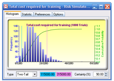
Figure 142.7: Statistical confidence levels
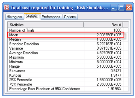
Figure 142.8: Simulated statistics