A very simple example is in order. Figure 16.2 illustrates the traveling financial planner problem. Suppose the traveling financial planner has to make three sales trips to New York, Chicago, and Seattle. Further, suppose that the order of arrival at each city is irrelevant. All that is important in this simple example is to find the lowest total cost possible to cover all three cities. Figure 16.2 also lists the flight costs from these different cities.
The problem here is cost minimization, suitable for optimization. One basic approach to solving this problem is through an ad hoc or brute force method. That is, manually list all six possible permutations as seen in Figure 16.3. Clearly, the cheapest itinerary is going from the east coast to the west coast, going from New York to Chicago, and finally on to Seattle. Here, the problem is simple and can be calculated manually, as there were three cities and, hence, six possible itineraries. However, add two more cities and the total number of possible itineraries jumps to 120. Performing an ad hoc calculation will be fairly intimidating and time-consuming. On a larger scale, suppose there are 100 cities on the salesman’s list; the possible itineraries will be as many as 9.3 x 10157. The problem will take many years to calculate manually, which is where optimization software steps in, automating the search for the optimal itinerary.
The example illustrated up to now is a deterministic optimization problem, that is, the airline ticket prices are known ahead of time and are assumed to be constant. Now suppose the ticket prices are not constant but are uncertain, following some distribution (e.g., a ticket from Chicago to Seattle averages $325, but is never cheaper than $300 and usually never exceeds $500). The same uncertainty applies to tickets for the other cities. The problem now becomes an optimization under uncertainty. Ad hoc and brute force approaches simply do not work. Software such as Risk Simulator can take over this optimization problem and automate the entire process seamlessly. The next section discusses the terms required in an optimization under uncertainty. The next chapter illustrates several additional business cases and models with step-by-step instructions.
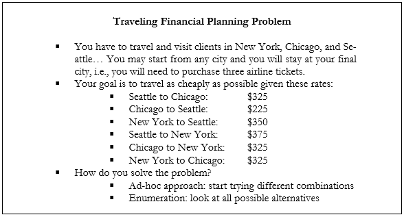
Figure 16.2: Traveling Financial Planner Problem
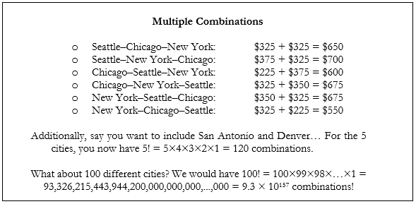
Figure 16.3: Multiple Combinations of the Traveling Financial Planner Problem