File Name: Decision Analysis – Decision Tree with EVPI, Minimax and Bayes’ Theorem
Location: Modeling Toolkit | Decision Analysis | Decision Tree with EVPI, Minimax and Bayes’ Theorem
Brief Description: Creates and solves a decision tree, applies Monte Carlo risk simulation on a decision tree, constructs a risk profile on a decision tree, computes Expected Value of Perfect Information, computes MINIMAX and MAXIMIN analysis, computes a Bayesian analysis on posterior probabilities, and aids in understanding the pros and cons of a decision tree analysis
Requirements: Modeling Toolkit, Risk Simulator
In this model, we create and value a decision tree using backward induction to make a decision on whether a Large, Medium, or Small facility should be built given uncertainties in the market. This model is intentionally set up such that it is generic and can be applied to any industry. For instance, in the oil and gas exploration and production application, “large, medium, and small” refers to the size of the drilling platform to be built, or in the manufacturing industry, these sizes refer to the size of a manufacturing facility to be built; in the real estate business, they refer to the size of the condominiums or quality (expensive, moderate, or low-priced housing), and so forth. In this model, we also determine if there is value in information, whether market research (the analogy in other industries would include wild cat exploratory wells, proof of concept development, initial research and development, and so forth) is worth anything and if it should be performed. In addition, other approaches are used including the MINIMAX and MAXIMIN computations, together with the application of Bayes’ Theorem (posterior updating on probabilities).
The problem is: A real estate developer (oil and gas exploration firm, manufacturing entity, research and development outfit, and others) is faced with the decision on whether to build Small, Medium, or Large condominiums. Clearly, the decision depends on how the market will be doing over the next few years, which is an unknown variable that may have a significant impact on the decision. The question is whether market research should be performed to obtain valuable information on how the market will be over the next few years as well as what the optimal decisions should be, given that the market research results can return either a Favorable or Unfavorable outcome. In consultation with marketing professionals and subject matter experts, the information in Figure 24.1 is generated and assumed to hold. For instance, the term Probability (Strong | Favorable) is the probability that the true outcome is a strong market given that a favorable rating is obtained through market research. The same convention is applied to the other probabilities.
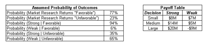
Figure 24.1: Payoff table and assumed probability of outcomes
A decision tree is then constructed using these inputs. That is, the initial decision is whether to invest in market research. If no market research is performed, the next step is to decide if a Small, Medium, or Large facility should be built. If market research is conducted, we wait for the results of the market research before deciding on whether to build the Small, Medium, or Large facility.
Decision Tree Construction and Solution
Using the assumptions just presented, a decision tree is built (Figure 24.2), based on chronological order, starting from the decision (a square box denotes a decision) of whether market research should be conducted or not. If no market research is performed, the next decision (another square box) is whether a Small, Medium, or Large facility should be built. Under each decision, the uncertainty of whether a Strong or Weak market exists is modeled (uncertainty outcomes are denoted by a circle), complete with its assumed probability of occurrence and payoff under each state of nature according to the assumptions above.
Next, the same construction is repeated with an intermediate step of performing the market research and waiting on the results (Favorable or Unfavorable). The decision on whether to build the Small, Medium, or Large facility now depends on the results of the market research, but all possible outcomes are enumerated, including their probabilities of occurrence and payoff levels according to the assumptions above.
The expected values are then computed on the tree as shown in Figure 24.2 (e.g., 7.94 is computed by taking 94% × 8 + 6% × 7, or 13.46 is computed by taking 94% × 14 + 6% x 5, and 18.26 is computed by taking the MAX [7.94, 13.46, 18.26] to find the optimal decision given a Favorable market research outcome). The optimal path is then listed in bold on the decision tree. The expected value is then worked all the way back to obtain 15.93 for market research (77% × 18.26 + 23% × 8.15) and 14.20 for no market research (computed through MAX [7.80, 12.20, 14.20] to find the optimal decision given no research).
Clearly, the higher expected value is 15.93, that is, to perform the market research. Further, if the market research results show a Favorable condition, the optimal decision is to build a Large facility. Conversely, build a Medium facility if an Unfavorable result is obtained.
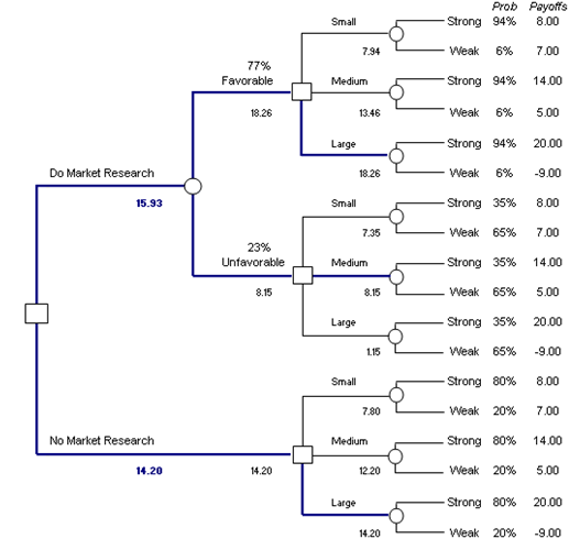
Figure 24.2: Decision tree construction
Monte Carlo Simulation on Decision Trees
The assumptions used in a decision tree are single-point estimates and may not be precise. The payoff values and probabilities are simply estimations at best. Hence, these single-point estimates can be enhanced through Risk Simulator’s Monte Carlo simulation. For the basic input assumptions, subject matter experts can be tasked with obtaining a most likely single-point estimate result while at the same, time, providing minimum and maximum estimates of each payoff and probability. These estimates are then entered into a Monte Carlo simulation (Figures 24.3, 24.4, and 24.5).
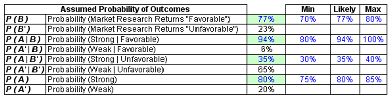
Figure 24.3: Probabilistic simulation assumption
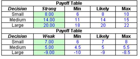
Figure 24.4: Payoff tables
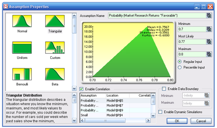
Figure 24.5: Running a simulation
The model already has these assumptions preset. To run the simulation, simply:
- Click on Risk Simulator | Change Profile and select the Decision Tree EVPI Minimax profile to open the simulation profile.
- Go to the Model worksheet and click on Risk Simulator | Run Simulation or click on the Run icon to run the simulation.
The forecast result of the Expected Value of Imperfect Information (cell R30) is shown in Figure 24.6, which is also the value of the difference between the expected value of performing market research and not performing market research. The forecast chart can be used to determine the probability that performing market research is better than not having any research. Further, the forecast chart shows that there is a 79.80% probability that doing market research is better than not doing any market research (select Right Tail on the forecast chart, enter in 0 on the left tail input box, and hit TAB on the keyboard). The expected value or mean of the distribution is 0.9736, indicating that the Expected Value of Imperfect Information is worth $0.9736M, which is the maximum amount of money the firm should spend, on average, to perform the market research. Further, the forecast chart on the Bayesian Posterior Probability (cell H60) indicates that the 95% confidence interval is between 87.83% and 97.69%. This means that on a 95% statistical basis (which means you are 95% sure) the results from the market research provide an accuracy of between 87.83% and 97.69%. That is, if the research results indicate that the market is strong, there is an 87.83% to 97.69% level of accuracy that the market is actually strong in reality. These computations are clearly seen in the Excel model.
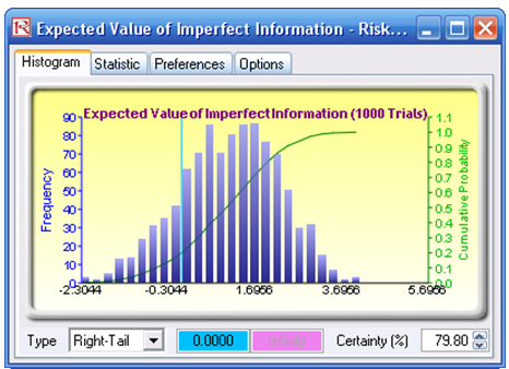
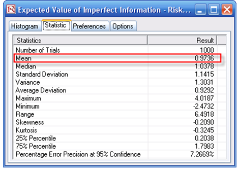
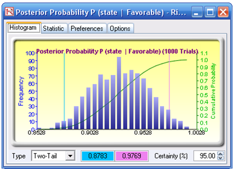
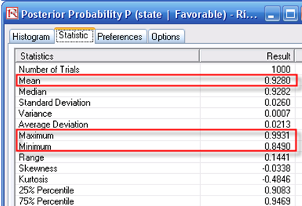
Figure 24.6: Simulation results
Risk Profile and EVPI
A risk profile based on the optimal path in the decision tree can be constructed. Specifically, comparing between not doing any market research versus performing the research, and looking at the optimal decision pathways, we obtain the results shown in Figure 24.7. 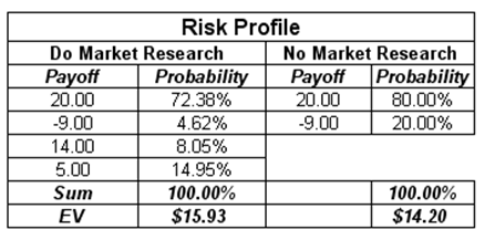
Figure 24.7: Risk-return profile
Notice that the expected values (EV) from the risk profile are exactly those in the decision tree (i.e., $15.93M and $14.20M), indicative of the two values from the optimal paths. Further, note that there is an 80% probability of making money ($20M) versus a 20% chance of losing money (-$9M) without the market research. In contrast, the risk profile has changed such that the chance of making a positive payoff is 95.38% (i.e., 72.38% + 8.05% + 14.95%) as compared to 4.62% of possibly losing money. Clearly, doing the research adds positive value to the project.
The difference between these two values, or $1.73M, is the Expected Value of Imperfect Information (EVII), that is, the value of the market research on a single-point estimate basis. This is termed “Imperfect Information” because no market research is perfect or provides the true result 100% of the time. There will clearly be some uncertainty left over.
Further, the Expected Value of Perfect Information (EVPI) can be obtained by computing the expected value of perfect information given the states of nature and the expected value of imperfect information given the states of nature and taking their differences (Figure 24.8). EVPI assumes that the information from the market research is 100% exact and precise.
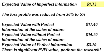
Figure 24.8: Expected value of perfect information
MAXIMIN and MINIMAX Analysis
MAXIMIN means maximizing the minimum outcomes. Specifically, looking at the no research strategy, the minimum payoffs (i.e., in the Weak states of nature), the maximum value is $7M (comparing among $7M, $5M, and -$9M). Therefore, using the MAXIMIN approach, a Small facility should be developed (Figure 24.9).
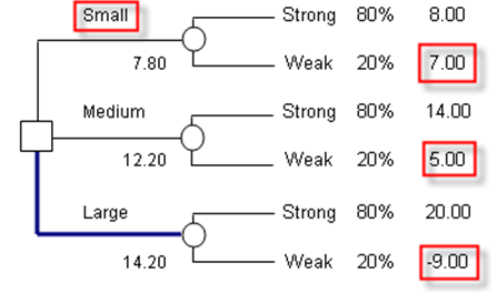
Figure 24.9: Maximin approach
In contrast, using the MINIMAX approach of minimizing the maximum regret, we see that the Medium facility should be built (Figures 24.10 and 24.11). The MINIMAX is computed by first obtaining the opportunity cost or regret matrix. For instance, if we built a Small facility, either a Strong or Weak market can exist. If a Strong market exists, we obtain $8M in payoff, but had we made a Large facility instead, the payoff would have been $20M. Therefore, you regret your decision as you could have made an additional $12M. Continuing with the analysis, a MINIMAX matrix is obtained for each state of nature. The Maximum of these regrets in all states of nature is computed for each decision. The Minimum is then computed. In this case, the result points to $6M or to build the Medium facility.
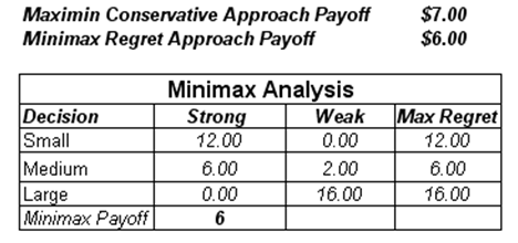
Figure 24.10: Minimax approach
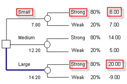
Figure 24.11: Minimax decision tree
Bayesian Analysis
Using the Bayes’ Theorem (Figure 24.12) and given that we have the information determined from expert opinions in consultation with the marketing professionals in Figure 24.13, we can derive the posterior probabilities.
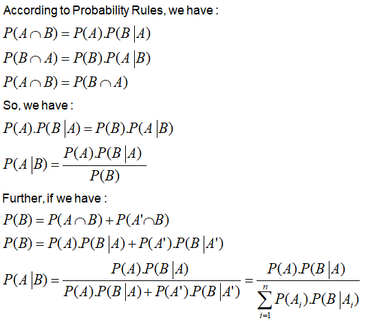
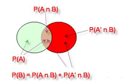
Figure 24.12: Intersection and union rules and graphical representation of probability theory
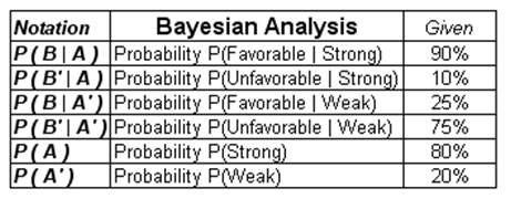
Figure 24.13: Input assumptions in a Bayes’ computation
To simplify, we denote A as the state of nature (A for Strong, and A′ for Weak), while we set B as the Favorable (B) or Unfavorable (B′) outcomes from the marketing research activities.
Using these rules, we can compute the Joint Probability P(B ∩ A) and the Bayes’ Posterior Probability P(A | B) as seen in Figure 24.14.
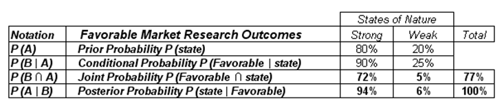
Figure 24.14: Bayes’ Theorem
That is, we have:
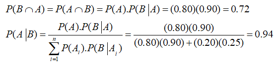
This means that market research holds significant value. If the research returns a Favorable judgment, there is a 94% probability of the true state of nature being Strong, and so forth. Using Bayes’ Theorem, we can determine this posterior probability, showing that the probabilities of making correct decisions are significantly higher than leaving it to chance. That is, obtain a 94% chance of being right as compared to an 80% chance if no market research is performed. The analysis can be repeated for the Unfavorable market research outcome.
Pros and Cons of Decision Tree Analysis
As you can see, decision tree analysis can be somewhat cumbersome, with all the associated decision analysis techniques. In creating a decision tree, be careful of its pros and cons. Specifically:
Pros
- Easy to use, construct, and value. Drawing the decision tree merely requires an understanding of the basics (e.g., the chronological sequence of events, payoffs, probabilities, decision nodes, chance nodes, and so forth; the valuation is simply expected values going from right to left on the decision tree).
- Clear and easy exposition. A decision tree is simple to visualize and understand.
Cons
- Ambiguous inputs. The analysis requires single-point estimates of many variables (many probabilities and many payoff values), and sometimes it is difficult to obtain objective or valid estimates. In a large decision tree, these errors in estimations compound over time, making the results highly ambiguous. The proverbial problem of garbage-in-garbage-out is clearly an issue here. Monte Carlo simulation with Risk Simulator helps by simulating the uncertain input assumptions thousands of times, rather than relying on single-point estimates.
- Ambiguous outputs. The decision tree results versus MINIMAX and MAXIMIN results produce different optimal strategies as illustrated in this chapter. Using decision trees will not necessarily produce robust and consistent results. Great care should be taken.
- Difficult and confusing mathematics. To make the decision tree analysis more powerful (rather than simply relying on single-point estimates), we revert to using Bayes’ Theorem. From the decision tree example, using the Bayes’ Theorem to derive implied and posterior probabilities is not an easy task at all. At best it is confusing and at worst, extremely complex to derive.
- In theory, each payoff value faces a different risk structure on the terminal nodes. Therefore, it is theoretically correct only if the payoff values (which have to be in present values) are discounted at different risk-adjusted discount rates, corresponding to the risk structure at the appropriate nodes. Obtaining a single valid discount rate is difficult enough, let alone multiple discount rates.
- The conditions, probabilities, and payoffs should be correlated to each other in real life. In a simple decision tree, this is not possible as you cannot correlate two or more probabilities. This is where Monte Carlo simulation comes in because it allows you to correlate pairs of input assumptions in a simulation.
- Decision trees do not solve real options Be careful as real options analysis requires binomial and multinomial lattices and trees to solve, not decision trees. Decision trees are great for framing strategic real options pathways but not for solving real options values. For instance, decision trees cannot be used to solve a switching option, or barrier option or option to expand, contract, and abandon. The branches on a decision tree are outcomes, while the branches on a lattice in a real option are options, not obligations. They are very different animals, so be extremely careful. In fact, Parts II and III are devoted to solving advanced real options problems, complete with explanations, examples, models, and case studies, clearly indicating that real options analysis is a lot more powerful and correct rather than using decision trees in solving most decisions under uncertainty and risk.