This technical note briefly explains the probability density function (PDF) for continuous distributions, which is also called the probability mass function (PMF) for discrete distributions (we use these terms interchangeably), where given some distribution and its parameters, we can determine the probability of occurrence given some outcome or random variable x. In addition, the cumulative distribution function (CDF) can also be computed, which is the sum of the PDF values up to this x value. Finally, the inverse cumulative distribution function (ICDF) is used to compute the value x given the cumulative probability of occurrence.
In mathematics and Monte Carlo risk simulation, a probability density function (PDF) represents a continuous probability distribution in terms of integrals. If a probability distribution has a density of f (x), then, intuitively, the infinitesimal interval of [x, x + dx] has a probability of f (x)dx. The PDF, therefore, can be seen as a smoothed version of a probability histogram; that is, by providing an empirically large sample of a continuous random variable repeatedly, the histogram using very narrow ranges will resemble the random variable’s PDF. The probability of the interval between [a, b] is given by ![]() which means that the total integral of the function f must be 1.0.
which means that the total integral of the function f must be 1.0.
It is a common mistake to incorrectly think of f (a) as the probability of a. In fact, f (a) can sometimes be larger than 1 (consider a uniform distribution between 0.0 and 0.5). The random variable x within this distribution will have f (x) greater than 1. The probability, in reality, is the function f (x)dx discussed previously, where dx is an infinitesimal amount.
The cumulative distribution function (CDF) is denoted as F(x) = P(X ≤ x), indicating the probability of X taking on a less than or equal value to x. Every CDF is monotonically increasing, is continuous from the right, and at the limits has the following properties: ![]()
Further, the CDF is related to the PDF by ![]() where the PDF function f is the derivative of the CDF function f. In probability theory, a probability mass function, or PMF, gives the probability that a discrete random variable is exactly equal to some value. The PMF differs from the PDF in that the values of the latter, defined only for continuous random variables, are not probabilities; rather, its integral over a set of possible values of the random variable is a probability. A random variable is discrete if its probability distribution is discrete and can be characterized by a PMF.
where the PDF function f is the derivative of the CDF function f. In probability theory, a probability mass function, or PMF, gives the probability that a discrete random variable is exactly equal to some value. The PMF differs from the PDF in that the values of the latter, defined only for continuous random variables, are not probabilities; rather, its integral over a set of possible values of the random variable is a probability. A random variable is discrete if its probability distribution is discrete and can be characterized by a PMF.
Therefore, X is a discrete random variable if
![]()
as u runs through all possible values of the random variable X.
INTERPRETING PROBABILITY CHARTS
Here are some tips to help decipher the characteristics of a distribution when looking at different PDF and CDF charts:
- For each distribution, a continuous distribution’s PDF is shown as an area chart (Figure TN.1) whereas a discrete distribution’s PMF is shown as a bar chart (Figure TN.2).
- If the distribution can only take a single shape (e.g., normal distributions are always bell shaped, with the only difference being the central tendency measured by the mean and the spread measured by the standard deviation), then typically only one PDF area chart will be shown with an overlay PDF line chart (Figure TN.3) showing the effects of various parameters on the distribution.
- The CDF charts, or S-Curves, are shown as line charts (Figure TN.4), and sometimes as bar graphs.
- The central tendency of a distribution(e.g., the mean of a normal distribution) is its central location (Figure TN.3).
- Multiple area charts and line charts will be shown (e.g., beta distribution) if the distribution can take on multiple shapes (e.g., the beta distribution is a uniform distribution when alpha = beta = 1; a parabolic distribution when alpha = beta = 2; a triangular distribution when alpha = 1 and beta = 2, or vice versa; a positively skewed distribution when alpha = 2 and beta = 5, and so forth). In this case, you will see multiple area charts and line charts (Figure TN.5).
- The starting point of the distribution is sometimes its minimum parameter (e.g., parabolic, triangular, uniform, arcsine, etc.) or its location parameter (e.g., the beta distribution’s starting location is 0, but a beta 4 distribution’s starting point is the location parameter; Figure TN.5 shows a beta 4 distribution with location = 10, its starting point on the x-axis).
- The ending point of the distribution is sometimes its maximum parameter (e.g., parabolic, triangular, uniform, arcsine, etc.) or its natural maximum multiplied by the factor parameter shifted by a location parameter (e.g., the original beta distribution has a minimum of 0 and maximum value of 1, but a beta 4 distribution with location = 10 and factor = 2 indicates that the shifted starting point is 10 and ending point is 11, and its width of 1 is multiplied by a factor of 2, which means that the beta 4 distribution now will have an ending value of 12, as shown in Figure TN.5).
- Interactions between parameters are sometimes evident. For example, in the beta 4 distribution, if the alpha = beta, the distribution is symmetrical, whereas it is more positively skewed the greater the difference between beta and alpha, and the more negatively skewed, the greater the difference between alpha and beta (Figure TN.6).
- Sometimes a distribution’s PDF is shaped by two or three parameters called shape and scale. For instance, the Laplace distribution has two input parameters, alpha location and beta scale, where alpha indicates the central tendency of the distribution (like the mean in a normal distribution) and beta indicates the spread from the mean (like the standard deviation in a normal distribution).
- The narrower the PDF(Figure TN.3’s normal distribution with a mean of 10 and standard deviation of 2), the steeper the CDF S-Curve looks (Figure TN.4), and the smaller the width on the CDF curve.
- A 45-degree straight line CDF(an imaginary straight line connecting the starting and ending points of the CDF) indicates a uniform distribution; an S-Curve CDF with equal amounts above and below the 45-degree straight line indicates a symmetrical and somewhat bell- or mound-shaped curve; a CDF completely curved above the 45-degree line indicates a positively skewed distribution (Figure TN.7), while a CDF completely curved below the 45-degree line indicates a negatively skewed distribution (Figure TN.8).
- A CDF line that looks identical in shape but shifted to the right or left indicates the same distribution but shifted by some location, and a CDF line that starts from the same point but is pulled both to the left and right indicates a multiplicative effect on the distribution such as a factor multiplication, as shown in Figures TN.9 and TN.10.
- An almost vertical CDF indicates a high kurtosis distribution with fat tails, and where the center of the distribution is pulled up (e.g., see the Cauchy distribution) versus a relatively flat CDF, a very wide and perhaps flat-tailed distribution is indicated.
- Some discrete distributions can be approximated by a continuous distribution if its number of trials is sufficiently large and its probability of success and failure is fairly symmetrical (e.g., see the binomial and negative binomial distributions). For instance, with a small number of trials and a low probability of success, the binomial distribution is positively skewed, whereas it approaches a symmetrical normal distribution when the number of trials is high, and the probability of success is around 0.50.
- Many distributions are both flexible and interchangeable––refer to the details of each distribution in the Test Driving Risk Simulator chapter’s appendices and Technical Note 2––e.g., binomial is Bernoulli repeated multiple times; arcsine and parabolic are special cases of beta; Pascal is a shifted negative binomial; binomial and Poisson approach normal at the limit; chi-square is the squared sum of multiple normal; Erlang is a special case of gamma; exponential is the inverse of the Poisson but on a continuous basis; F is the ratio of two chi-squares; gamma is related to the lognormal, exponential, Pascal, Erlang, Poisson, and chi-square distributions; Laplace comprises two exponential distributions in one; the log of a lognormal approaches normal; the sum of multiple discrete uniforms approach normal; Pearson V is the inverse of gamma; Pearson VI is the ratio of two gammas; PERT is a modified beta; a large degree of freedom T approaches normal; Rayleigh is a modified Weibull; and so forth.
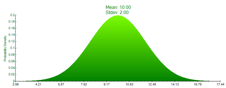
Figure TN.1: Continuous PDF (Area Chart)
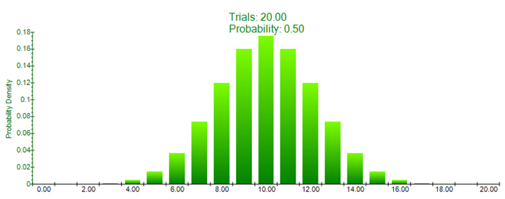
Figure TN.2: Discrete PMF (Bar Chart)
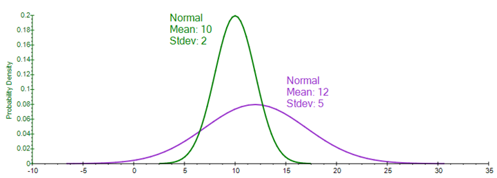
Figure TN.3: Multiple Continuous PDF Overlay Charts
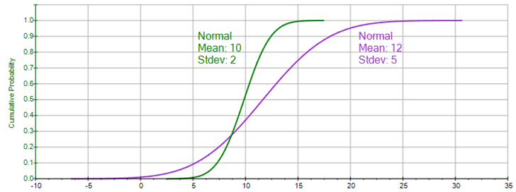
Figure TN.4: CDF Overlay Charts
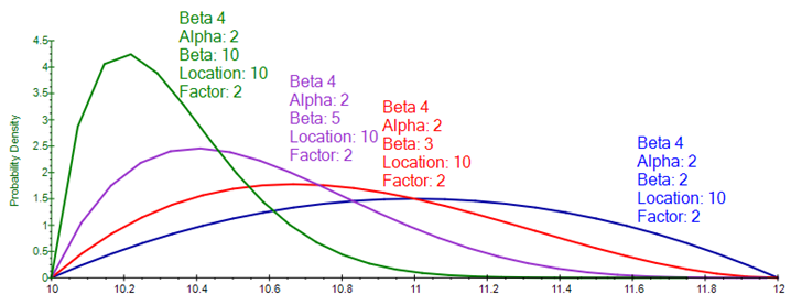
Figure TN.5: PDF Characteristics of the Beta Distribution
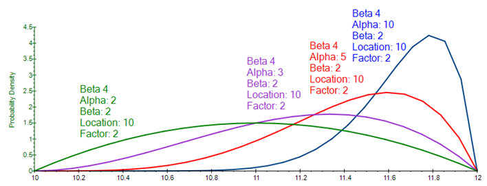
Figure TN.6: PDF of a Negatively Skewed Beta Distribution
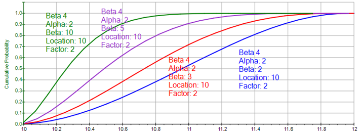
Figure TN.7: CDF of a Positively Skewed Distribution
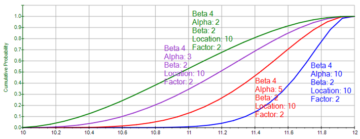
Figure TN.8: CDF of a Negatively Skewed Distribution
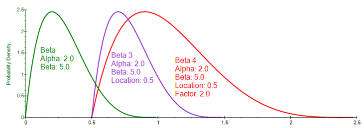
Figure TN.9: PDF Characteristics of a Shift
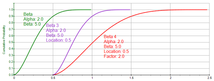
Figure TN.10: CDF Characteristics of a Shift