Theory
A hypothesis test is performed when testing the means and variances of two distributions to determine if they are statistically identical or statistically different from one another; that is, to see if the differences between the means and variances of two different forecasts that occur are based on random chance or if they are, in fact, statistically significantly different from one another.
This analysis is related to bootstrap simulation but with several differences. Classical hypothesis testing uses mathematical models and is based on theoretical distributions. This means that the precision and power of the test are higher than bootstrap simulation’s empirically based method of simulating a simulation and letting the data tell the story. However, classical hypothesis tests are only applicable for testing two distributions’ means and variances (and by extension, standard deviations) to see if they are statistically identical or different. In contrast, nonparametric bootstrap simulation can be used to test for any distributional statistics, making it more useful, but the drawback is its lower testing power. Risk Simulator provides both techniques from which to choose.
Procedure
- Run Simulation (e.g., use the Risk Simulator | Example Models | 08 Hypothesis Testing and Bootstrap Simulation).
- Select Risk Simulator | Analytical Tools | Hypothesis Testing.
- Select the two forecasts to test, select the type of hypothesis test you wish to run, and click OK (Figure 15.18).
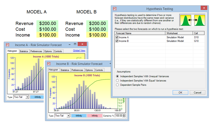
Figure 15.18: Hypothesis Testing
Results Interpretation
A two-tailed hypothesis test is performed on the null hypothesis (H0) such that the two variables’ population means are statistically identical to one another. The alternative hypothesis (Ha) is such that the population means are statistically different from one another. If the calculated p-values are less than or equal to 0.01, 0.05, or 0.10 alpha test levels, it means that the null hypothesis is rejected, which implies that the forecast means are statistically significantly different at the 1%, 5%, and 10% significance levels. If the null hypothesis is not rejected when the p-values are high, the means of the two forecast distributions are statistically similar to one another. The same analysis is performed on variances of two forecasts at a time using the pairwise F-test. If the p-values are small, then the variances (and standard deviations) are statistically different from one another, otherwise, for large p-values, the variances are statistically identical to one another. The example file used was Hypothesis Testing and Bootstrap Simulation (Figure 15.19).
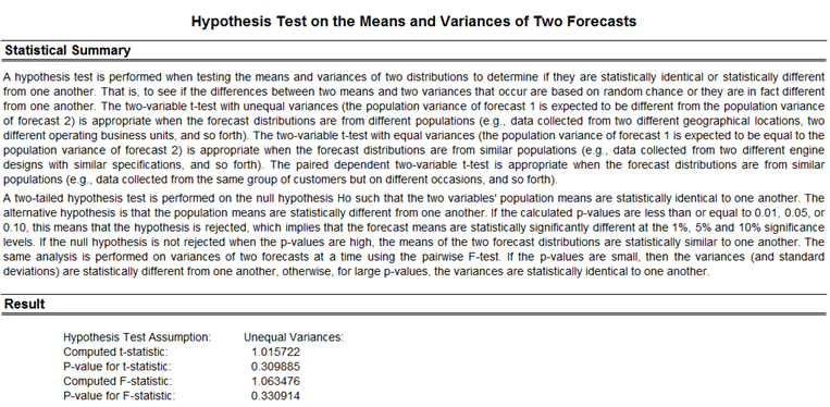
Figure 15.19: Hypothesis Testing Results
Notes
The two-variable t-test with unequal variances (the population variance of forecast 1 is expected to be different from the population variance of forecast 2) is appropriate when the forecast distributions are from different populations (e.g., data collected from two different geographical locations, or two different operating business units, and so forth). The two-variable t-test with equal variances (the population variance of forecast 1 is expected to be equal to the population variance of forecast 2) is appropriate when the forecast distributions are from similar populations (e.g., data collected from two different engine designs with similar specifications, and so forth). The paired dependent two-variable t-test is appropriate when the forecast distributions are from exactly the same population and subjects (e.g., data collected from the same group of patients before an experimental drug was used and after the drug was applied, and so forth).