File Name: Forecasting – Markov Chains and Market Share
Location: Modeling Toolkit | Forecasting | Markov Chains and Market Share
Brief Description: Illustrates how to run a simulation model on Markov chains to determine path-dependent movements of market share and the long-term steady-state effects of market share
Requirements: Modeling Toolkit, Risk Simulator
The Markov Process is useful for studying the evolution of systems over multiple and repeated trials in successive time periods. The system’s state at a particular time is unknown, and we are interested in knowing the probability that a particular state exists. For instance, Markov Chains are used to compute the probability that a particular machine or equipment will continue to function in the next time period or whether a consumer purchasing Product A will continue to purchase Product A in the next period or switch to a competitive brand B.
Procedure
- When opening this model, make sure to select Enable Macros when prompted (you will get this prompt if your security settings are set to Medium, i.e., click on Tools | Macros | Security | Medium when in Excel). The Model worksheet shows the Markov Process and is presented as a chain of events, also known as a Markov Chain.
- Enter the required inputs (i.e., values in blue: probabilities of switching or transition probabilities, the initial store location, and the number of periods to forecast using the Markov Process). Click Compute when ready.
Note: The probabilities are typically between 5% and 95%, and the Checksum total probabilities must be equal to 100%. These transition probabilities represent the probabilities that a customer will visit another store in the next period. For instance, 90% indicates that the customer is currently a patron of Store A and there is a 90% probability that s/he will stay at Store A the next period and 10% probability that s/he will be visiting another store (Store B) the next period. Therefore, the total probability must be equal to 100% (Figure 86.1).
- Further, select the location of the customer at time zero or right now, whether it is Store A or Store B.
- Finally, enter the number of periods to forecast, typically between 5 and 50 periods. You cannot enter a valueless than 1 or more than 1000.
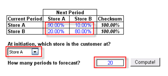
Figure 86.1: Markov chain input assumptions
Results
The results from a Markov Process include a chain of events, indicating the transition from one store to the next. For instance, if there are 1,000 customers total, at Period 5, there will be 723 customers, on average, in Store A versus 277 in Store B, and so forth. Over time, a steady state occurs, and the Steady State Probability results indicate what would happen if the analysis is performed over a much longer period. These steady-state probabilities are also indicative of the respective market shares. In other words, over time and at equilibrium, Store A has a 66.67% market share as compared to 33.33% market share (Figure 86.2).
Alternatively, you can use Risk Simulator’s Markov Chain forecasting module to automatically generate forecast values (Risk Simulator | Forecasting | Markov Chain).
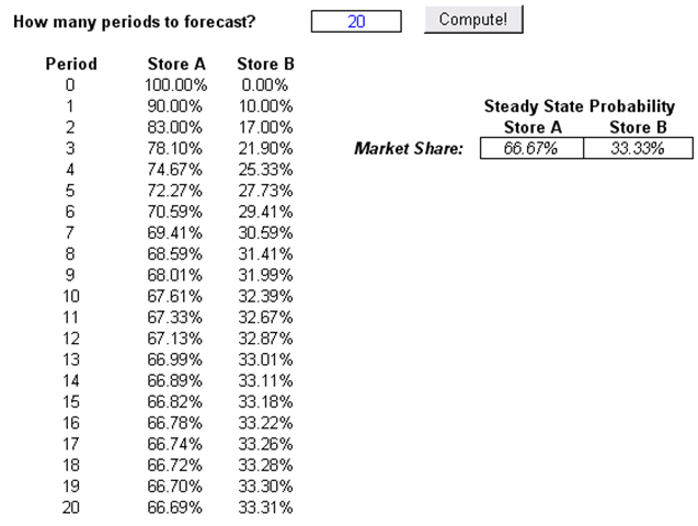
Figure 86.2: Markov chain results with steady-state effects
This analysis can be extended to, say, a machine functioning over time. In the example given, say the probability of a machine functioning in the current state will continue to function the next period about 90% of the time. Then the probability that the machine will still be functioning in 5 periods is 72.27% or 66.67% in the long run.