File Name: Forecasting – Time-Series Analysis
Location: Modeling Toolkit | Forecasting | Time Series Analysis
Brief Description: Illustrates how to run time-series analysis forecasts, which take into account historical base values, trends, and seasonalities to project the future
Requirements: Modeling Toolkit, Risk Simulator
The historical sales revenue data are located in the Time-series Data worksheet in the model. The data are quarterly sales revenue from Q1 2000 to Q4 2004. The data exhibit quarterly seasonality, which means that the seasonality is 4 (there are 4 quarters in 1 year or 1 cycle).
Time-series forecasting decomposes the historical data into the baseline, trend, and seasonality, if any. The models then apply an optimization procedure to find the alpha, beta, and gamma parameters for the baseline, trend, and seasonality coefficients, and then recompose them into a forecast. In other words, this methodology first applies a backcast to find the best-fitting model and best-fitting parameters of the model that minimizes forecast errors, and then proceeds to forecast the future based on the historical data that exist. This, of course, assumes that the same baseline growth, trend, and seasonality hold going forward. Even if they do not—say, when there exists a structural shift (e.g., company goes global, has a merger, spin-off, etc.)—the baseline forecasts can be computed, and then the required adjustments can be made to the forecasts.
Procedure
To run this model, simply:
- Select the historicaldata (cells H11:H30).
- Select Risk Simulator | Forecasting | Time-Series Analysis.
- Select Auto Model Selection, Forecast 4 Periods and Seasonality 4 Periods (Figure 91.1).
Note that you can select Create Simulation Assumptions only if an existing Simulation Profile exists. If not, click on Simulation | New Simulation Profile, and then run the time-series forecast per steps 1 to 3 above but remember to check the Create Simulation Assumptions box.
Model Results Analysis
For your convenience, the analysis Report and Methodology worksheets are included in the model. A fitted chart and forecast values are provided in the report as well as the error measures and a statistical summary of the methodology (Figure 91.2). The Methodology worksheet provides the statistical results from all eight time-series methodologies.
Several different types of errors can be calculated for time-series forecast methods, including the mean-squared error (MSE), root-mean-squared error (RMSE), mean absolute deviation (MAD), and mean absolute percent error (MAPE).
The MSE is an absolute error measure that squares the errors (the difference between the actual historical data and the forecast-fitted data predicted by the model) to keep the positive and negative errors from canceling each other out. This measure also tends to exaggerate large errors by weighting the large errors more heavily than smaller errors by squaring them, which can help when comparing different time-series models. The MSE is calculated by simply taking the average of the Error2. RMSE is the square root of MSE and is the most popular error measure, also known as the quadratic loss function. RMSE can be defined as the average of the absolute values of the forecast errors and is highly appropriate when the cost of the forecast errors is proportional to the absolute size of the forecast error.
MAD is an error statistic that averages the distance (absolute value of the difference between the actual historical data and the forecast-fitted data predicted by the model) between each pair of actual and fitted forecast data points. MAD is calculated by taking the average of the |Error| and is most appropriate when the cost of forecast errors is proportional to the absolute size of the forecast errors.
MAPE is a relative error statistic measured as an average percent error of the historical data points and is most appropriate when the cost of the forecast error is more closely related to the percentage error than the numerical size of the error. This error estimate is calculated by taking the average of

where Yt is the historical data at time t, while ![]() is the fitted or predicted data point at time t using this time-series method. Finally, an associated measure is the Theil’s U statistic, which measures the naivety of the model’s forecast. That is, if the Theil’s U statistic is less than 1.0, then the forecast method used provides an estimate that is statistically better than guessing. Figure 91.3 provides the mathematical details of each error estimate.
is the fitted or predicted data point at time t using this time-series method. Finally, an associated measure is the Theil’s U statistic, which measures the naivety of the model’s forecast. That is, if the Theil’s U statistic is less than 1.0, then the forecast method used provides an estimate that is statistically better than guessing. Figure 91.3 provides the mathematical details of each error estimate.
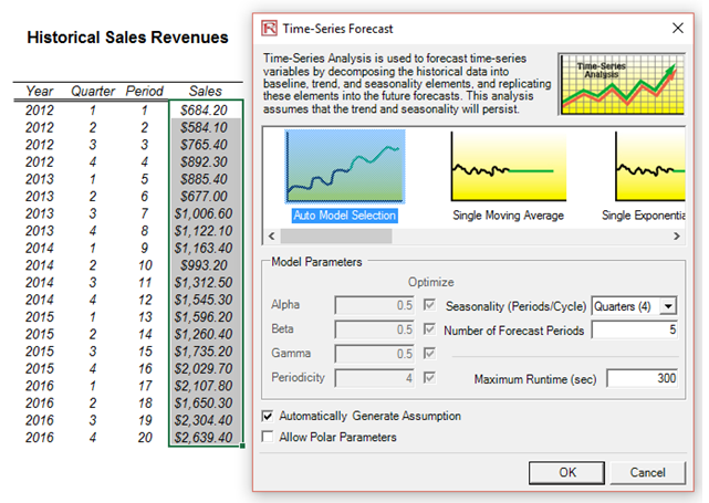
Figure 91.1: Running a time-series analysis forecast
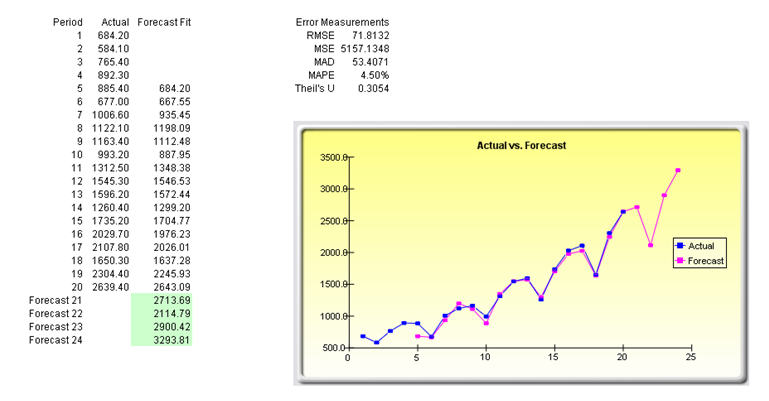
Figure 91.2: Time-series analysis results
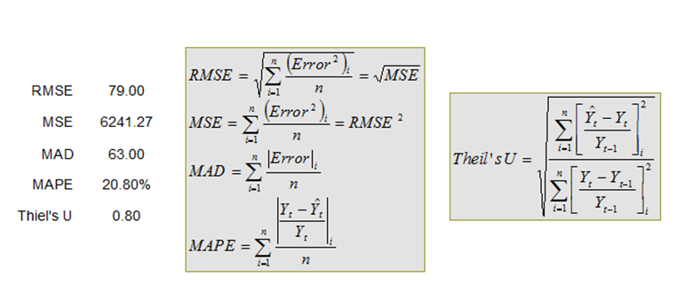
Figure 91.3: Error computations