File Name: Optimization – Military Portfolio and Efficient Frontier
Location: Modeling Toolkit | Optimization | Military Portfolio and Efficient Frontier
Brief Description: Illustrates how to run an optimization on discrete binary integer decision variables in project selection and mix; view and interpret optimization results; create additional qualitative constraints to the optimization model; and generate an investment Efficient Frontier by applying optimization on changing constraints
Requirements: Modeling Toolkit, Risk Simulator
This model shows 20 different projects with different risk-return characteristics as well as several qualitative measures such as strategic score, military readiness score, tactical score, comprehensive score, and so forth (see Figure 100.1). These scores are obtained through subject matter experts, for instance, decision makers, leaders, and managers of organizations, where their expert opinions are gathered through the double-blind Delphi Method. After being scrubbed (e.g., extreme values are eliminated, large data variations are analyzed, multiple iterations of the Delphi Method are performed, etc.), their respective scores can be entered into a Distributional Fitting routine to find the best-fitting distribution, or used to develop a Custom Distribution for each project.
The central idea of this model is to find the best portfolio allocation such that the portfolio’s total comprehensive strategic score and profits are maximized. That is, it is used to find the best project mix in the portfolio that maximizes the total Profit*Score measure, where profit points to the portfolio level net returns after considering the risks and costs of each project, while the Score measures the total comprehensive score of the portfolio, all the while being subject to the constraints on the number of projects, budget constraint, full-time equivalence resource (FTE) restrictions, and strategic ranking constraints.
Objective: Maximize Total Portfolio Returns times the Portfolio Comprehensive
Score (C28)
Decision Variables: Allocation or Go/No-Go Decision (J5:J24)
Restrictions on Decision Variables: Binary decision variables (0 or 1)
Constraints: Total Cost (E26) is less than or equal to $3800 (in $ thousand or $ million)
Less than or equal to 10 projects selected (J26) in the entire portfolio
Full-time Equivalence resources have to be less than or equal to 80 (M26)
Total Strategic Ranking for the portfolio must be less than or equal to 100 (F26)
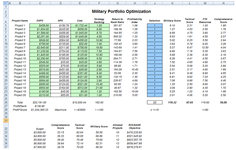
Figure 100.1: The project selection optimization model
Running an Optimization
To run this preset model, simply open the profile (Risk Simulator | Change Profile) and select Military Portfolio and Efficient Frontier. Then, run the optimization (Risk Simulator | Optimization | Run Optimization) or for practice, set up the model yourself:
- Start a new profile(Risk Simulator | New Profile) and give it a name.
- In this example, all the allocations are required to be binary (0 or 1) values, so, first select cell J5 and make this a decision variable in the Integer Optimization Select cell J5 and define it as a decision variable (Risk Simulator | Optimization | Set Decision or click on the Set Decision icon) and make it a Binary Variable. This setting automatically sets the minimum to 0 and maximum to 1 and can only take on a value of 0 or 1. Then use the Risk Simulator Copy on cell J5, select cells J6 to J24, and use Risk Simulator’s Paste (Risk Simulator | Copy Parameter and Risk Simulator | Paste Parameter or use the Risk Simulator copy and paste icons, NOT the Excel copy/paste).
- Next, set up the optimization’s constraints by selecting Risk Simulator | Optimization | Constraints, and select ADD. Then link to cell E26, and make it <= 3800, select ADD one more time and click on the link icon and point to cell J26 and set it to <=10. Continue with adding the other constraints (cell M26 <= 80 and F26 <= 100).
- Select cell C28, the objective to be maximized, Risk Simulator | Optimization | Set Objective, and then select Risk Simulator | Optimization | Run Optimization. Review the different tabs to make sure that all the required inputs in steps 2 and 3 above are correct.
- You may now select the optimization method of choice and click OK to run the optimization. The model setup is illustrated in Figure 100.2.
Note: If you are to run either a dynamic or stochastic optimization routine, make sure that first, you have assumptions defined in the model; that is, that some of the cells in C5:C24 and E5:F24 are assumptions. The suggestion for this model is to run a Discrete Optimization.
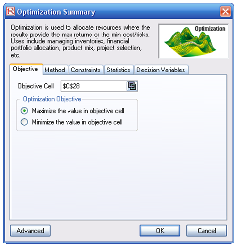
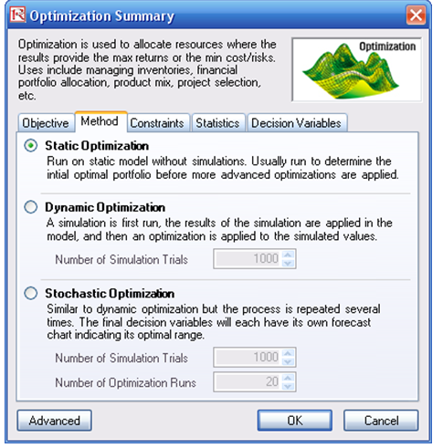
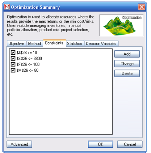
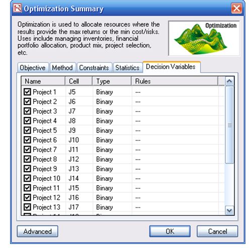
Figure 100.2: Setting up an optimization model
Portfolio Efficient Frontier
Clearly, running the optimization procedure will yield an optimal portfolio of projects where the constraints are satisfied. This represents a single optimal portfolio point on the efficient frontier, for example, Portfolio B on the chart in Figure 100.3. Then, by subsequently changing some of the constraints, for instance, by increasing the budget and allowed projects, we can rerun the optimization to produce another optimal portfolio given these new constraints. Therefore, a series of optimal portfolio allocations can be determined and graphed. This graphical representation of all optimal portfolios is called the Portfolio Efficient Frontier. At this juncture, each point represents a portfolio allocation, for instance, Portfolio B might represent projects 1, 2, 5, 6, 7, 8, 10, 15, and so forth, while Portfolio C might represent projects 2, 6, 7, 9, 12, 15, and so forth, each resulting in different tactical, military, or comprehensive scores and portfolio returns. It is up to the decision maker to decide which portfolio represents the best decision and if sufficient resources exist to execute these projects.
Typically, in an Efficient Frontier analysis, you would select projects where the marginal increase in benefits is positive, and the slope is steep. In the next example, you would select Portfolio D rather than Portfolio E as the marginal increase is negative on the y-axis (e.g., Tactical Score). That is, spending too much money may actually reduce the overall tactical score, and hence this portfolio should not be selected. Also, in comparing Portfolios A and B, you would be more inclined to choose B as the slope is steep and the same increase in budget requirements (x-axis) would return a much higher percentage Tactical Score (y-axis). The decision to choose between Portfolios C and D would depend on available resources and the decision maker deciding if the added benefits warrant and justify the added budget and costs.
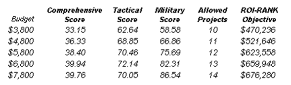
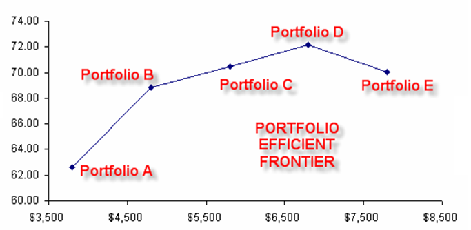
Figure 100.3: Efficient frontier
To further enhance the analysis, you can obtain the optimal portfolio allocations for C and D and then run a simulation on each optimal portfolio to decide what the probability that D will exceed C in value is, and whether this probability of occurrence justifies the added costs.
If you’re in college perhaps you’re thinking which person you should contact to aid you with writing an essay. There are a variety of resources to help, should you require an essay to be used in a certain class or have trouble https://www.sfweekly.com/sponsored/review-of-the-top-5-academic-assistance-platforms/ understanding the topic. Many students do not have the necessary skills for writing an intriguing piece that will distinguish themselves from others. Here are some methods to find someone who can assist you.