Generally, forecasting can be divided into quantitative and qualitative approaches. Qualitative forecasting is used when little to no reliable historical, contemporaneous, or comparable data exist. Several qualitative methods exist such as the Delphi or expert opinion approach (a consensus-building forecast by field experts, marketing experts, or internal staff members), management assumptions (target growth rates set by senior management), as well as market research or external data or polling and surveys (data obtained through third-party sources, industry and sector indexes, or active market research). These estimates can be either single-point estimates (an average consensus) or a set of prediction values (a distribution of predictions). The latter can be entered into Risk Simulator as a custom distribution and the resulting predictions can be simulated; that is, running a nonparametric simulation using the prediction data points as the custom distribution.
For quantitative forecasting, the available data or data that need to be forecasted can be divided into time-series (values that have a time element to them, such as revenues at different years, inflation rates, interest rates, market share, failure rates, and so forth), cross-sectional (values that are time-independent, such as the grade point average of sophomore students across the nation in a particular year, given each student’s levels of SAT scores, IQ, and the number of alcoholic beverages consumed per week), or mixed panel (a mixture between time-series and panel data, e.g., predicting sales over the next 10 years given budgeted marketing expenses and market share projections, which means that the sales data are time-series but exogenous variables such as marketing expenses and market share exist to help to model the forecast predictions).
Here is a quick review of each methodology and several quick getting started examples in using the software. More detailed descriptions and example models of each of these techniques are found throughout this and the next chapter.
- ARIMA. Autoregressive integrated moving average (ARIMA, also known as Box–Jenkins ARIMA) is an advanced econometric modeling technique. ARIMA looks at historical time-series data and performs back-fitting optimization routines to account for historical autocorrelation (the relationship of a variable’s values over time, that is, how a variable’s data is related to itself over time), accounts for the stability of the data to correct for the nonstationary characteristics of the data, and learns over time by correcting its forecasting Think of ARIMA as an advanced multiple regression model on steroids, where time-series variables are modeled and predicted using its historical data as well as other time-series explanatory variables. Advanced knowledge in econometrics is typically required to build good predictive models using this approach. Suitable for time-series and mixed-panel data (not applicable for cross-sectional data).
- Auto ARIMA. The Auto-ARIMA module automates some of the traditional ARIMA models by automatically testing multiple permutations of model specifications and returns the best-fitting Running the Auto-ARIMA module is similar to running regular ARIMA forecasts. The differences being that the required P, D, Q inputs in ARIMA are no longer required and that different combinations of these inputs are automatically run and compared. Suitable for time-series and mixed-panel data (not applicable for cross-sectional data).
- Basic Econometrics. Econometrics refers to a branch of business analytics, modeling, and forecasting techniques for modeling the behavior or forecasting certain business, economic, finance, physics, manufacturing, operations, and any other variables. Running the Basic Econometrics models is similar to regular regression analysis except that the dependent and independent variables are allowed to be modified before a regression is run. Suitable for all types of data.
- Basic Auto Econometrics. This methodology is similar to basic econometrics, but thousands of linear, nonlinear, interacting, lagged, and mixed variables are automatically run on your data to determine the best-fitting econometric model that describes the behavior of the dependent variable. It is useful for modeling the effects of the variables and for forecasting future outcomes, while not requiring the analyst to be an expert econometrician. Suitable for all types of data.
- Combinatorial Fuzzy Logic. Fuzzy sets deal with approximate rather than accurate binary logic. Fuzzy values are between 0 and 1. This weighting schema is used in a combinatorial method to generate the optimized time-series forecast Suitable for time-series data only.
- Custom Distributions. Using Risk Simulator, expert opinions can be collected, and a customized distribution can be generated. This forecasting technique comes in handy when the dataset is small when the Delphi method is used, or the goodness-of-fit is bad when applied to a distributional fitting Suitable for all types of data.
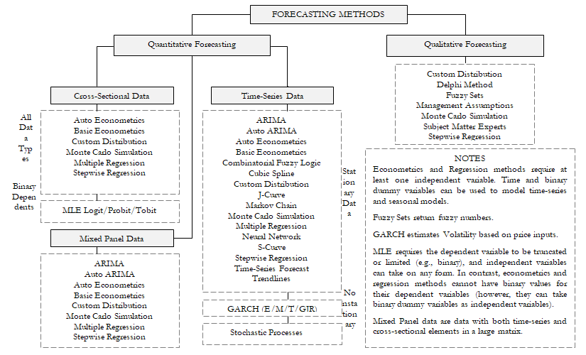
Figure 11.1: Forecasting Methods
- GARCH. The generalized autoregressive conditional heteroskedasticity(GARCH) model is used to model historical and forecast future volatility levels of a marketable security (e.g., stock prices, commodity prices, oil prices, etc.). The dataset has to be a time series of raw price levels. GARCH will first convert the prices into relative returns and then run an internal optimization to fit the historical data to a mean-reverting volatility term structure, while assuming that the volatility is heteroskedastic in nature (changes over time according to some econometric characteristics). Several variations of this methodology are available in Risk Simulator, including EGARCH, EGARCH-T, GARCH-M, GJR-GARCH, GJR-GARCH-T, IGARCH, and T-GARCH. Suitable for time-series data only.
- J-Curve. The J-curve, or exponential growth curve, is one where the growth of the next period depends on the current period’s level and the increase is exponential. This phenomenon means that over time, the values will increase significantly, from one period to another. This model is typically used in forecasting biological growth and chemical reactions over time. Suitable for time-series data only.
- Markov Chains. A Markov chain exists when the probability of a future state depends on a previous state and when linked together forms a chain that reverts to a long-run steady-state level. This approach is typically used to forecast the market share of two competitors. The required inputs are the starting probability of a customer in the first store (the first state) returning to the same store in the next period, versus the probability of switching to a competitor’s store in the next state. Suitable for time-series data only.
- Maximum Likelihood on Logit, Probit, and Tobit. Maximum likelihood estimation(MLE) is used to forecast the probability of something occurring given some independent variable For instance, MLE is used to predict if a credit line or debt will default given the obligor’s characteristics (30 years old, single, salary of $100,000 per year, and total credit card debt of $10,000), or the probability a patient will have lung cancer if the person is a male between the ages of 50 and 60, smokes five packs of cigarettes per month or year, and so forth. In these circumstances, the dependent variable is limited (i.e., limited to being binary 1 and 0 for default/die and no default/live, or limited to integer values such as 1, 2, 3, etc.) and the desired outcome of the model is to predict the probability of an event occurring. Traditional regression analysis will not work in these situations (the predicted probability is usually less than zero or greater than one, and many of the required regression assumptions are violated, such as independence and normality of the errors, and the errors will be fairly large). Suitable for cross-sectional data only.
- Multivariate Regression. Multivariate regression is used to model the relationship structure and characteristics of a certain dependent variable as it depends on other independent exogenous variables. Using the modeled relationship, we can forecast the future values of the dependent variable. The accuracy and goodness-of-fit for this model can also be determined. Linear and nonlinear models can be fitted in the multiple regression analysis. Suitable for all types of data.
- Neural Network. This method creates artificial neural networks, nodes, and neurons inside software algorithms for the purposes of forecasting time-series variables using pattern recognition. Suitable for time-series data
- Nonlinear Extrapolation. In this methodology, the underlying structure of the data to be forecasted is assumed to be nonlinear over time. For instance, a dataset such as 1, 4, 9, 16, 25 is considered to be nonlinear (these data points are from a squared function). Suitable for time-series data only.
- S-Curves. The S-curve, or logistic growth curve, starts off like a J-curve, with exponential growth rates. Over time, the environment becomes saturated (e.g., market saturation, competition, overcrowding), the growth slows, and the forecast value eventually ends up at a saturation or maximum level. The S-curve model is typically used in forecasting market share or sales growth of a new product from market introduction until maturity and decline, population dynamics, and other naturally occurring phenomena. Suitable for time-series data only.
- Spline Curves. Sometimes there are missing values in a time-series For instance, interest rates for years 1 to 3 may exist, followed by years 5 to 8, and then year 10. Spline curves can be used to interpolate the missing years’ interest rate values based on the data that exist. Spline curves can also be used to forecast or extrapolate values of future time periods beyond the time period of available data. The data can be linear or nonlinear. Suitable for time-series data only.
- Stochastic Process Forecasting. Sometimes variables are stochastic and cannot be readily predicted using traditional Nonetheless, most financial, economic, and naturally occurring phenomena (e.g., the motion of molecules through the air) follow a known mathematical law or relationship. Although the resulting values are uncertain, the underlying mathematical structure is known and can be simulated using Monte Carlo risk simulation. The processes supported in Risk Simulator include Brownian motion random walk, mean-reversion, jump-diffusion, and mixed processes, useful for forecasting nonstationary time-series variables. Suitable for time-series data only.
- Time-Series Analysis and Decomposition. In well-behaved time-series data (typical examples include sales revenues and cost structures of large corporations), the values tend to have up to three elements: a base value, trend, and seasonality. Time-series analysis uses these historical data and decomposes them into these three elements, and recomposes them into future forecasts. In other words, this forecasting method, like some of the others described, first performs a back-fitting (backcast) of historical data before it provides estimates of future values (forecasts). Suitable for time-series data only.
- Trendlines. This method fits various curves such as linear, nonlinear, moving average, exponential, logarithmic, polynomial, and power functions on existing historical data. Suitable for time-series data only.